R E S E A R C H
Open Access
A posteriori
error estimates for the
fractional optimal control problems
Xingyang Ye
1and Chuanju Xu
2**Correspondence: [email protected] 2School of Mathematical Sciences,
Xiamen University, Xiamen, 361005, China
Full list of author information is available at the end of the article
Abstract
In this paper, we study the spectral approximation for a constrained optimal control problem governed by the time fractional diffusion equation.A posteriorierror estimates are obtained for both the state and the control approximations. Some numerical experiments are carried out to show that the obtaineda posteriorierror estimates are reliable.
Keywords: fractional optimal control problem; space-time spectral method; a posteriorierror
1 Introduction
Optimal control problems have been subject of many research works in scientific and en-gineering computing. The literature on this field is huge, and it is impossible to give even a very brief review. It has been found that the fractional order model can provide a more realistic description for some kind of complex systems in the fields covering control the-ory [], viscoelastic materials [, ], anomalous diffusion [–], advection and dispersion of solutes in porous or fractured media [],etc.[–]. Consequently, an optimal control problem for fractional differential equations initiates a new research direction, and we see a growing interest in this topic from both scientific and engineering communities.
A general formulation and a solution scheme for the fractional optimal control prob-lem (FOCP) were first proposed in [], where the fractional variational principle and the Lagrange multiplier technique were used. Following this idea, Frederico and Torres [] formulated a Noether-type theorem in the general context and studied fractional con-servation laws. Mophou [] applied the classical control theory to a fractional diffusion equation, involving a Riemann-Liouville fractional time derivative. Dorvilleet al.[] later extended the results of [] to a boundary fractional optimal control.
Recently, some efforts have been put into developing spectral methods for solving FOCPs. For instance, a numerical direct method based on the Legendre orthonormal ba-sis and operational matrix of Riemann-Liouville fractional integration were introduced in [] to solve a general class of FOCP, and the convergence of the proposed method was also extensively discussed. In [], the Legendre spectral-collocation method was applied to obtain approximate solutions for some types of FOCPs. Ye and Xu [] proposed a Galerkin spectral method to solve a linear quadratic FOCP associated with the time frac-tional diffusion equation with Caputo fracfrac-tional derivative, and a detailed error analysis was carried out. However, to the best of our knowledge, much less research is available for
thea posteriori error estimation for problems involving fractional derivative, especially the one for FOCP.
The purpose of this paper is to derivea posteriorierror estimates for the FOCP gov-erned by the time fractional diffusion equation (TFDE) with Riemann-Liouville fractional derivative. Let= (–, ),I= (,T),=×I. We consider the following linear-quadratic optimal control problem for the control variablequnder constraints:
min
q∈K
u(x,t) –u¯(x,t)dxdt+λ
q(x,t) dxdt
, (.)
whereλandu¯are given,uis governed by the TFDE as follows:
R
∂tαu(x,t) –∂xu(x,t) =f(x,t) +q(x,t), ∀(x,t)∈, I–α
t u(x, ) = , ∀x∈, (.)
u(–,t) =u(,t) = , ∀t∈I,
withR∂tα( <α< ) denoting the left Riemann-Liouville fractional derivative,It–α denot-ing the Riemann-Liouville fractional integral, and
K=
q∈L() :
q(x,t) dxdt≥
.
The main physical purpose for adopting and investigating diffusion equations of frac-tional order is to describe phenomena of anomalous diffusion usually met in transport processes through complex and/or disordered systems including fractal media []. In [], Nigmatullin used the fractional diffusion equation to describe diffusion in media with fractal geometry. Mainardi [] pointed out that the propagation of mechanical diffusive wave in viscoelastic media can be modeled by TFDE. An interesting review on the anoma-lous diffusion by Metzler and Klafter [] has appeared to which (and references therein) we refer the interested reader. Applying a time fractional integration of orderα to both sides of the first equation in (.) allows us to eliminate the time fractional derivative on the L.H.S. leading to the integral form
u(x,t) – (α)
t
∂
xu(x,τ) (t–τ)–αdτ=
(α)
t
f(x,τ) +q(x,τ)
(t–τ)–α dτ. (.)
The outline of the paper is as follows. In the next section we discuss the optimality con-ditions and spectral discretization of the optimal problem.A posteriorierror estimate is derived in Section . Finally, in Section , we carry out some numerical tests to verify the theoretical results.
For a domainO, which may be,Ior, we useL(O),Hs(O), andHs
(O) to denote the
usual Sobolev spaces, equipped with the norms · ,O and · s,O respectively. For the
Sobolev spaceXwith the norm · X, we define the spaceHs(I;X) :={v|v(·,t)X∈Hs(I)} endowed with the normvHs(I;X):=v(·,t)Xs,I. Particularly, whenXstands forHμ() orHμ(), the norm of the spaceHs(I;X) will be denoted by ·
2 Optimization and spectral approximation of the problem
For a weak formula of the state equation (.), we introduce the control spaceL() and
the state space []
Bs() =HsI,L()∩LI,H(), ∀s> ,
equipped with the norm
vBs()=v
Hs(I,L())+vL(I,H ())
.
Then a weak formulation for the state equation (.) reads as follows: givenq,f ∈L(), findu∈Bα() such that
A(u,v) = (f +q,v), ∀v∈B
α
(), (.)
where the bilinear formA(·,·) is defined by
A(u,v) :=R∂
α
t u,Rt∂
α
Tv
+ (∂xu,∂xv).
Here, R
∂
α
t andRt∂
α
T respectively denote the left and right Riemann-Liouville fractional derivatives of order α.
By defining the cost functional
J(q,u) := u–u¯
,+
λ q
,, (q,u)∈K×B
α
(), (.)
with the given desired stateu¯∈L(), the optimal control problem reads as follows: find (q∗,u(q∗))∈K×Bα() such that
Jq∗,uq∗= min
(q,u)∈K×Bα()
J(q,u) subject to (.). (.)
The well-posedness of the state problem ensures the existence of a control-to-state map-pingq→u=u(q) defined through (.). By means of this mapping we introduce the re-duced cost functionalJ:L()→Ras follows:
J(q) :=Jq,u(q), q∈L().
Then the optimal control problem (.) is equivalent to findingq∗∈Ksuch that
Jq∗=min
q∈KJ(q). (.)
The first order necessary optimality condition for (.) reads
Jq∗δq–q∗≥, ∀δq∈K, (.)
It has been proved [] that
J(q)(δq) =λq+z(q),δq, ∀δq∈L(), (.)
wherez(q) =z∈Bα() is the solution of the following adjoint state equation:
A(ϕ,z) = (u–u¯,ϕ), ∀ϕ∈B
α
(). (.)
Now, we consider the spectral approximation of the optimal control problem. We define the polynomial space
PM() =PM()∩H(), SL=PM()⊗PN(I)⊂Bα(),
wherePMdenotes the space of all polynomials of degree less than or equal toM,Lstands for the parameter pair (M,N).
Then we consider the spectral approximation to the state equation (.) as follows: find uL(q)∈SLsuch that
AuL(q),vL
= (f+q,vL), ∀vL∈SL. (.)
Similar to the continuous case, we introduce the semidiscrete reduced cost functional JL:L()→Ras follows:
JL(q) :=Jq,uL(q), q∈L(), (.)
whereuL(q) is given by (.). Then we consider the following auxiliary optimal problem: findq∗∈Ksuch that
JLq∗=min
q∈KJL(q). (.)
The solutionq∗of the above problem fulfills the first order optimality condition
JLq∗δq–q∗≥, ∀δq∈K, (.)
where
JL(q)(φ) =λq+zL(q),φ, ∀q,φ∈K, (.)
withzL(q)∈SLbeing the solution of the semidiscrete adjoint problem
AϕL,zL(q)
=uL(q) –u¯,ϕL
, ∀ϕL∈SL. (.)
Now we consider the approximation of the control space to obtain the full discrete op-timal control problem. To this end, we introduce the finite dimensional subspace for the control variable as follows:
Then the full discrete optimal control problem reads as follows: findq∗L∈KLsuch that
JLq∗L= min
qL∈KLJL(qL), (.)
where JL(·) is defined in (.). The unique solution of (.),q∗L, satisfies the following optimality condition:
JLq∗Lδq–q∗L≥, ∀δq∈KL. (.)
3 A posteriori error estimates
We aim in this section at deriving estimates of the error between a continuous solution and its spectral approximation in terms of known and computable quantities,i.e.,a poste-riorierror estimates. We will confine ourselves to the so-called residual-based estimates []. To simplify the notations, we letcbe a generic positive constant independent of any functions and of any discretization parameters. We use the expressionABto mean that A≤cB.
The error analysis will make use of some projection operators. The orthogonal projector ,M :H
()→PM() is defined by∀v∈H(), ,
Mv∈PM() such that
,Mv–v,φM = , ∀φM∈PM().
The following estimates hold []:∀v∈Hm()∩H(),m≥,
,
Mv–v,M
–mv m,, ,
Mv–v,M
–mv m,.
For theL-orthogonal projectorN, defined byNv∈PN(I), such that (Nv–v,wN)I= ,∀wN∈PN(I), we have
Nv–v,IN–mvm,I, ∀v∈Hm(I),m≥.
TheL-orthogonal projectorMinis defined similarly.
The first step is to derivea posteriorierror estimates for the approximation to the control variable.
Lemma . Suppose q∗and q∗Lare the solutions of (.)and(.)respectively,then the following estimate holds:
q∗–q∗L,zLq∗L–zq∗L,, (.)
where zL(q∗L)and z(qL∗)are respectively the solutions of (.)and(.)associated to q∗L.
Proof Similar to Lemma . in [], it follows from (.), (.) and (.) that for allp,q∈ L(),
Then in virtue of (.) and (.) we get, for arbitrarypL∈KL,
λq∗–q∗L,
≤Jq∗q∗–q∗L–JqL∗q∗–q∗L ≤–JqL∗q∗–q∗L
=JLq∗LqL∗–q∗–Jq∗Lq∗–q∗L+JLq∗Lq∗–qL∗
=JLq∗LqL∗–pL+JLq∗LpL–q∗
–λqL∗+zq∗L,q∗–q∗L+λq∗L+zL
q∗L,q∗–q∗L
≤JLq∗LpL–q∗+zLq∗L–zq∗L,q∗–q∗L
=zLqL∗+λqL∗,pL–q∗+zLq∗L–zq∗L,q∗–q∗L. (.)
Furthermore, as shown in Lemma in [], it holds
zL
q∗L+λq∗L,MNq∗–q∗
= . (.)
Therefore, by takingpL=NMq∗in (.), then using (.) and the Cauchy-Schwarz
in-equality, we obtain (.).
Theorem . Let q∗be the solution of(.),u(q∗)and z(q∗)be the corresponding state and the adjoint state respectively.Let q∗Lbe the solution of(.)with the corresponding discrete state uL(q∗L)and the adjoint state zL(q∗L).Then the following estimate holds:
q∗–q∗L,+uq∗–uLq∗L
Bα()+z
q∗–zLq∗L
Bα()η+η,
where
η=
N–α +M–ξ, η=N–α +M–ξ,
with
ξ=Rt∂TαzL
q∗L–∂xzL
q∗L–uL
q∗L+u¯,,
ξ=R∂
α tuL
q∗L–∂xuLqL∗–f –q∗L,.
Proof We first estimateq∗–q∗L,. According to (.), it suffices to estimatezL(q∗L) – z(q∗L),. Letez=zL(qL∗) –z(q∗L),eLz =N,Mez∈SL. It follows from (.) and (.) that
AeLz,ez
=uL
q∗L–uqL∗,eLz.
It has been proved [] that for allu,v∈Bα(), the following continuity and coercivity
hold:
A(u,v)u
Bα()vBα(), A(v,v)v
Thus, using (.), (.), (.), and (.), we have
zLq∗L–zq∗L Bα()
A(ez,ez) =A
ez–eLz,ez
+AeLz,ez
=Aez–eLz,zLq∗L–Aez–eLz,zq∗L+AeLz,ez
=R∂
α
t
ez–eLz,Rt∂
α
TzL
q∗L+∂x
ez–eLz,∂xzLq∗L
–uq∗L–u¯,ez–eLz+uLq∗L–uq∗L,eLz
=ez–eLz,Rt∂TαzLq∗L–ez–eLz,∂xzLq∗L–uq∗L–u¯,ez–eLz
+uL
q∗L–uqL∗,eLz–ez
+
uL
q∗L–uq∗L,ez
=ez–eLz,Rt∂TαzLq∗L–∂xzLq∗L+uLq∗L–u¯,eLz –ez
+uLq∗L–uq∗L,ez
=ez–eLz,Rt∂TαzL
q∗L–∂xzL
q∗L–uL
q∗L+u¯
+uLq∗L–uq∗L,ez
ez–eLz,ξ+uL
qL∗–uq∗L,ez,. (.)
Furthermore,
ez–eLz,
≤ ez–Nez,+Nez–N,Mez,
≤ ez–Nez,+N
ez–,Mez–ez–,Mez,
+ez–,Mez,
ez–Nez,+ez–,Mez,
N–αe
z,α,+M–ez,,
N–αez
Bα()+M –ez
Bα(). (.)
Plugging (.) into (.) yields
zLq∗L–zq∗L
Bα()η+uL
q∗L–uq∗L,. (.)
Similarly, seteu=uL(q∗L) –u(q∗L), and leteLu=N,Meu∈SL. Then it follows from (.) and (.) thatA(eu,eL
u) = , and thus
uLq∗L–uq∗L Bα()
A(eu,eu) =Aeu,eu–eLu
=AuL
q∗L,eu–eLu
–Auq∗L,eu–eLu
ξeu–eLu,
ξ
N–αeu
,α,+M–eu,,
ξ
N–α +M–eu
Bα().
This leads to
uL
q∗L–uq∗L
Bα()η. (.)
Then combining (.) and (.) gives
zLq∗L–zq∗L
Bα()η+uL
q∗L–uq∗L,η+η.
Using the above estimate, the inequality · , ·
Bα(), and Lemma ., we get
q∗–q∗L,η+η. (.)
Furthermore, using the triangle inequalities
zL
q∗L–zq∗
Bα()≤zL
q∗L–zq∗L
Bα()+z
qL∗–zq∗ Bα(),
uLq∗L–uq∗
Bα()≤uL
q∗L–uq∗L
Bα()+u
q∗L–uq∗ Bα(),
and the following obvious estimates
zq∗L–zq∗
Bα()u
q∗L–uq∗,q∗L–q∗,,
we obtain
uLq∗L–uq∗
Bα()+zL
q∗L–zq∗
Bα()η+η.
This completes the proof.
4 Optimization algorithm and numerical results 4.1 Projection gradient optimization algorithm
In what follows, we propose a projection gradient optimization algorithm to solve the resulting minimization problems. The key of the algorithm is to determine a suitable pro-jector to guarantee that the imposed constraint on the control variable is satisfied. To this end, to anyqL∈PM()⊗PN(I) we associate the functionqK= –min{,qL}+qLsuch that qK∈K.
Then we propose the following projection gradient algorithm for the optimal control problem (.):
• Start with an initial controlq()L . • Repeat fork= , , . . ..
- Update:q(k+
)
L =q
(k)
L –ρkJL(q
(k)
L ).
- Projection:q(k+
)
L →q
(k+)
L :=q
(k+)
K .
• Until stopping criterion is satisfied.
The proposed stopping criterion is
JLq(Lk)≤ε, (.)
where εis a pre-defined tolerance. Whenever (.) is satisfied for somek, the optimal control variableq∗Lis supposed to be obtained,i.e.,q∗L=q(Lk).
The key components of the above algorithm include:
(i) Determination of the descent direction. (ii) Choice of the step size.
The details are described below. Given an initial controlq()L , the corresponding state uL(q()L ) is given by the solution of the state equation in (.). To apply the stopping cri-terionJL(q()L ) ≤ε, we need information on the adjoint statezL(q()L ), which is obtained from the adjoint state equation (.) for givenuL(q()L ) andq()L . Then the descent direc-tion, that is, the gradient of the objective functional atq()L , is calculated through
dL():=JLq()L =zL
q()L +λq()L .
Then, assuming knownq(Lk)anddL(k)at the current (kth) iteration, we updateq(Lk)via
q(k+
)
L =q
(k)
L –ρkd
(k)
L , q
(k+)
L = –min ,q
(k+)
L
+q(k+
)
L ,
whereρkis the iteration step size determined in a way such that
JLq(Lk)–ρkd(Lk)=min
ρ>JL
q(Lk)–ρd(Lk).
Such aρkis characterized by
z(k+
)
L +λ
q(Lk)–ρkdL(k),dL(k)= , (.)
wherez(k+
)
L ∈SLis the solution of
AϕL,z
(k+)
L
=u(k+
)
L –u¯,ϕL
, ∀ϕL∈SL (.)
withu(k+
)
L ∈SLgiven by
Au(k+
)
L ,vL
=f +q(Lk)–ρkdL(k),vL, ∀vL∈SL. (.)
The optimal iteration step sizeρkcan be efficiently calculated through solving (.).
In-deed we first notice that there exists an explicit expression ofz(k+
)
L onρk. Letu˜
(k)
L andz˜
(k)
L denote respectively the solutions of
AϕL,z˜(Lk)
=u˜(Lk),ϕL
, ∀ϕL∈SL. (.)
uL(q(Lk)) andzL(q(Lk)) are respectively the solutions of
AuL
q(Lk),vL
=f+q(Lk),vL
, ∀vL∈SL, (.)
AϕL,zL
q(Lk)=uL
q(Lk)–u¯,ϕL
, ∀ϕL∈SL. (.)
Then it can be checked thatzL(q(Lk)) –ρk˜z(Lk)solves (.) and (.), that is,
z(k+
)
L =zL
q(Lk)–ρkz˜(Lk).
Bringing this expression into (.) gives
zLq(Lk)–ρkz˜(Lk)+λ
q(Lk)–ρkdL(k),dL(k)= .
Letd˜(Lk)=˜zL(k)+λd(Lk), then we obtain
ρk=
(d(Lk),d(Lk)) (d˜(Lk),d(Lk))
. (.)
The overall process is summarized below.
Projection gradient optimization algorithm Choose an initial controlq()L , setk= .
(a) Solve problems (.) and (.), letdL(k)=zL(qL(k)) +λq(Lk).
(b) Solve problems (.) and (.), and setd˜(Lk)=˜zL(k)+λd(Lk),ρk=
(dL(k),d(Lk))
(d˜L(k),d(Lk))
.
(c) Update:q(k+
)
L =q
(k)
L –ρkd
(k)
L ,q
(k+)
L = –min{,q
(k+)
L }+q
(k+)
L .
(d) Ifd(Lk) ≤tolerance, then takeq∗L=q(Lk+)and solve problems (.) and (.) to get
uL(q∗L)andzL(q∗L).
Else, setk=k+ , repeat (a)-(d).
4.2 Numerical results
In this subsection we carry out some numerical experiments to validate thea posteriori error estimates for the numerical solutions. In our calculation, we takeT= ,λ= .
Example . We consider problem (.) with exact analytical solutions as
uq∗=sinπxcosπt, zq∗=sinπxsinπ( –t), q∗=max ,zq∗–zq∗. The right-hand sidef and the desired stateu¯here are respectively numerically calculated through (.) and (.) usingu(q∗),z(q∗) andq∗.
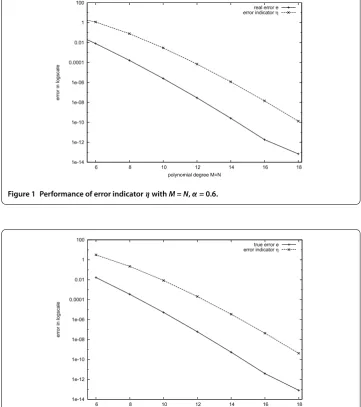
In order to validate the a posteriori error estimate, we compare the error indicator η=η+η, which is defined in Theorem . and the real error of the numerical solution
measured by
e=q∗–qL∗,+uq∗–uLq∗L
Bα()+z
Figure 1 Performance of error indicatorηwithM=N,α= 0.6.
Figure 2 Performance of error indicatorηwithM=N,α= 0.3.
These two errors are compared in Figure as functions ofM(=N). We observe that the indicatorηhas almost the same exponential decay as the errore, whereas it overestimates the error, which is consistent with our theoretical results.
Example . We choose other exact analytical solutions as
uq∗=sinπxet, zq∗=sinπx( –t)et, q∗=max ,zq∗–zq∗.
5 Concluding remarks
We have obtaineda posterioriupper bound of the spectral method for the fractional con-trol problem. This is an important step towards developing an adaptive spectral method for solving FOCPs. In the future, we will consider the efficiency of thea posteriori estima-tor to obtain an optimal estimate. As for the classical parabolic equation, we guess such an optimal estimate will have to make use of some Jacobi-weighted Sobolev spaces and polynomial inverse inequalities. Furthermore, many computational issues have to be ad-dressed. For example, an adaptive refinement strategy should be investigated for efficiently implementing the adaptive spectral method for FOCPs, and the adaptive spectral method should be also used to solve some real examples from physical and engineering sciences.
Competing interests
The authors declare that they have no competing interests.
Authors’ contributions
The authors have equal contributions to each part of this paper. All the authors read and approved the final manuscript.
Author details
1School of Science, Jimei University, Xiamen, 361021, China.2School of Mathematical Sciences, Xiamen University,
Xiamen, 361005, China.
Acknowledgements
The work of XY Ye is partially supported by the Science Foundation of Jimei University, China (Grant Nos. ZQ2013005 and ZC2013021), the Foundation (Class B) of Fujian Educational Committee (Grant No. FB2013005), the Foundation of Fujian Educational Committee (No. JA14180). The work of CJ Xu was partially supported by the National NSF of China (Grant Nos. 11471274 and 11421110001).
Received: 11 November 2014 Accepted: 9 April 2015
References
1. Oustaloup, A: La Dérivation Non Entière: Théorie, Synthèse et Applications. Hermes, Paris (1995)
2. Koeller, RC: Application of fractional calculus to the theory of viscoelasticity. J. Appl. Mech.51, 299-307 (1984) 3. Mainardi, F: Fractional diffusive waves in viscoelastic solids. In: Nonlinear Waves in Solids, pp. 93-97 (1995) 4. Bouchaud, JP, Georges, A: Anomalous diffusion in disordered media: statistical mechanisms, models and physical
applications. Phys. Rep.195(4-5), 127-293 (1990)
5. Dentz, M, Cortis, A, Scher, H, Berkowitz, B: Time behavior of solute transport in heterogeneous media: transition from anomalous to normal transport. Adv. Water Resour.27(2), 155-173 (2004)
6. Goychuk, I, Heinsalu, E, Patriarca, M, Schmid, G, Hänggi, P: Current and universal scaling in anomalous transport. Phys. Rev. E73(2), 020101 (2006)
7. Benson, DA, Wheatcraft, SW, Meerschaert, MM: The fractional-order governing equation of Lévy motion. Water Resour. Res.36(6), 1413-1423 (2000)
8. Diethelm, K: The Analysis of Fractional Differential Equations. Springer, Berlin (2010)
9. Miller, K, Ross, B: An Introduction to the Fractional Calculus and Fractional Differential Equations. Wiley, New York (1993)
10. Podlubny, I: Fractional Differential Equations. Academic Press, New York (1999)
11. Agrawal, O: A general formulation and solution scheme for fractional optimal control problems. Nonlinear Dyn.38(1), 323-337 (2004)
12. Frederico, G, Torres, D: Fractional optimal control in the sense of Caputo and the fractional noethers theorem. Int. Math. Forum3(10), 479-493 (2008)
13. Mophou, GM: Optimal control of fractional diffusion equation. Comput. Math. Appl.61(1), 68-78 (2011)
14. Dorville, R, Mophou, GM, Valmorin, VS: Optimal control of a nonhomogeneous Dirichlet boundary fractional diffusion equation. Comput. Math. Appl.62(3), 1472-1481 (2011)
15. Lotfi, A, Yousefi, S, Dehghan, M: Numerical solution of a class of fractional optimal control problems via the Legendre orthonormal basis combined with the operational matrix and the Gauss quadrature rule. J. Comput. Appl. Math.250, 143-160 (2013)
16. Sweilam, N, Al-Ajami, T: Legendre spectral-collocation method for solving some types of fractional optimal control problems. J. Adv. Res. (2014). doi:10.1016/j.jare.2014.05.004
17. Ye, XY, Xu, C: A spectral method for optimal control problems governed by the time fractional diffusion equation with control constraints. In: Spectral and High Order Methods for Partial Differential Equations (ICOSAHOM 2012), pp. 403-414. Springer, Berlin (2014)
18. Gorenflo, R, Mainardi, F, Moretti, D, Paradisi, P: Time fractional diffusion: a discrete random walk approach. Nonlinear Dyn.29(1-4), 129-143 (2002). doi:10.1023/A:1016547232119
19. Nigmatullin, RR: The realization of the generalized transfer equation in a medium with fractal geometry. Phys. Status Solidi B133(1), 425-430 (1986)
20. Metzler, R, Klafter, J: The random walk’s guide to anomalous diffusion: a fractional dynamics approach. Phys. Rep.
21. Li, XJ, Xu, CJ: A space-time spectral method for the time fractional diffusion equation. SIAM J. Numer. Anal.47(3), 2108-2131 (2009)
22. Canuto, C, Hussaini, MY, Quarteroni, A, Zang, TA: Spectral Methods - Fundamentals in Single Domains. Springer, Berlin (2006)