Analysis of a stochastic predator–prey population model with Allee effect and jumps

R E S E A R C H

Open Access

Analysis of a stochastic predator–prey

population model with Allee effect and jumps

Rong Liu

_{and Guirong Liu}

*_{Correspondence:}

[email protected]

1_{School of Mathematical Sciences,} Shanxi University, Taiyuan, P.R. China

Abstract

This paper is concerned with a stochastic predator–prey model with Allee effect and Lévy noise. First, by the comparison theorem of stochastic differential equations, we prove that the model has a unique global positive solution starting from the positive initial value. Then we investigate the asymptotic pathwise behavior of the model by the generalized exponential martingale inequality and the Borel–Cantelli lemma. Next, we establish the conditions under which predator and prey populations are extinct. Furthermore, we show that the global positive solution is stochastically ultimate bounded under some conditions by using the Bernoulli equation and Chebyshev’s inequality. At last, we introduce some numerical simulations to support the main results obtained. The results in this paper generalize and improve the previous related results.

MSC: 60H10; 60J60; 92D25; 92D40

Keywords: Allee effect; Lévy noise; Exponential martingale inequality; Chebyshev’s inequality; Predator–prey

1 Introduction

The dynamic relationship between predators and their preys has been universal in both ecology and mathematical ecology [1,2]. The classic predator–prey population model is the Lotka–Volterra model established by Alfred James Lotka and Vito Volterra in the 1920s. There are many extensive studies in the literature concerned with the dynamics of the predator–prey models and we here do not mention them in detail. However, for the last decade, the importance of the Allee effect has been recognized. Because of the diffi-culties in finding mates when the prey population density becomes low, the Allee effect may occur in prey species [3]. For example, this might correspond to the density below which it is so difficult to find a mate that reproduction does not compensate for mortal-ity. In [4], the authors studied the following deterministic predator–prey population with Allee effect on prey:

⎧ ⎨ ⎩

dx(t) dt =x(t)[

bx(t)

A1+x(t)–d1–αx(t) –

sy(t) 1+sh1x(t)], dy(t)

dt =y(t)[ c1sx(t) 1+sh1x(t)–d2],

(1.1)

with initial valuesx(0) =x0,y(0) =y0. Herex(t) andy(t) represent, respectively, the size of prey and predator population at timet;b is the per capita maximum fertility rate of

prey population;di(i= 1, 2) are the per capita death rates of prey and predators,

respec-tively;αdenotes the strength of the intra-competition of the prey population;sdenotes the effective search rate;h1 denotes the handling time of predators; andc1denotes the conversion efficiency of ingested prey into new predators. The product, ₁₊sx_sh1x(t)_(t), repre-sents the predator’s functional response. All the parameters of the model are supposed to be positive constants.

It is well known that populations in nature are inevitably subjected to various types of environmental noise. During the past decades, a great deal of attention has been paid to the study of stochastic biological models (see [5–9]). In [10], the authors perturb the death ratesd1of prey andd2of the predator population in (1.1) with Gaussian white noise and obtain the following stochastic predator–prey population model:

⎧ ⎨ ⎩

dx(t) =x(t)[_A1bx₊(_xt₍)_t)–d1–αx(t) –₁₊sy_sh1x(t)_(t)] dt–σ1x(t) dw1(t), dy(t) =y(t)[₁₊c1sx_sh1x(t₍)_t)–d2] dt–σ2y(t) dw2(t).

(1.2)

However, biological systems may suffer sudden environmental shocks: such as earth-quakes, toxic pollutants, hurricanes and so on. Note that these sudden environmental shocks will cause jumps in the population dynamics. As mentioned in [11], here a jump means a sudden shift on the size of biological population, and the mathematical explana-tion is that sample paths are not continuous almost surely. It is recognized that stochastic differential equations with Lévy noise are quite suitable to describe such a discontinu-ous system. Recently, stochastic differential equations with Lévy processes have been re-searched widely both in theory and their applications [12–16]. References [13] and [14] are devoted to the stochastic Lotka–Volterra population dynamics with jumps, and the former with a stochastic competitive Lotka–Volterra model, and the latter with a general Lotka–Volterra model. In [15], the authors studied the asymptotic behavior of a stochastic population model with Allee effect and Lévy jumps.

Motivated by the above discussion, in this paper, we consider the following stochastic predator–prey model with Allee effect and Lévy jumps:

⎧ ⎪ ⎪ ⎪ ⎪ ⎪ ⎨ ⎪ ⎪ ⎪ ⎪ ⎪ ⎩

dx(t) =x(t–)[_A1bx₊(_xt₍–)_t–)–d1–αx(t–) –₁₊sy_sh1x(t–)_(t–)] dt –σ1x(t–) dw1(t) –

Γ γ1(u)x(t–)N˜(dt, du),

dy(t) =y(t–)[₁₊c1sx_sh1x(t₍–)_t–)–d2] dt–σ2y(t–) dw2(t) –_Γγ2(u)y(t–)N˜(dt, du),

(1.3)

with initial valuesx(0) =x0,y(0) =y0. Herex(t–) is the left limit ofx(t) andy(t–) is the left limit ofy(t). All meanings of the parameters are exact as or similar to those for (1.1) except the following.w(t) ={w1(t),w2(t)}represents a standard two-dimensional Brow-nian motion defined on a compete probability space (Ω,F,P) with a filtration{Ft}t≥0 satisfying the usual conditions (i.e. it is right continuous andF0contains allP-null sets).

N(·,·) is a Poisson counting process with characteristic measureλon measurable subset

Γ of [0,∞) withλ(Γ) <∞. Then the compensated Poisson random measureN(dt, du) =

N(dt, du) –λ(du) dtis a martingale, which is independent ofw(t). Usually, the pair (w,N) is called Lévy noise. Throughout this paper, we denoteR2

The remainder of the present paper is organized as follows. First, in Sect.2, we prove that this model has a unique global positive solution starting from the positive initial value by the comparison theorem of stochastic differential equations. In Sect.3, we investigate the asymptotic pathwise behavior of the model by using the generalized exponential martin-gale inequality and the Borel–Cantelli lemma. Extinction conditions of the population will be established in Sect.4. In Sect.5, we show that the global positive solution is stochas-tically ultimate bounded under some conditions. Section6contains numerical results, which are used to demonstrate the effectiveness of the theoretical results in this paper. The paper ends with a conclusion.

2 Existence and uniqueness of positive solution

In this section, by using comparison theorem of stochastic differential equations, we show that system (1.3) has a unique positive global solution with positive initial value. For sim-plicity, we introduce the following notation:

βi=

σ2

i

2 –

Γ

ln1 –γi(u)

+γi(u)

λ(du), i= 1, 2.

Note thatγi(u) < 1 onΓ. Thus, for anyu∈Γ, we have 1 –γi(u) > 0. By the basic inequality x– 1 –lnx≥0 forx> 0, we have

– γi(u) +ln

1 –γi(u)

=1 –γi(u)

– 1 –ln1 –γi(u)

≥0 foru∈Γ.

Thus,βi= σ_i2

2 –

Γ[ln(1 –γi(u)) +γi(u)]λ(du)≥ σ_i2

2 > 0,i= 1, 2. Moreover, we assume that there is a constantK> 0 such that

Γ

ln1 –γi(u)

2

λ(du) <K, i= 1, 2. (2.1)

Theorem 2.1 For any given initial value(x0,y0)∈R2+,system(1.3)has a unique global

positive solution(x(t),y(t))on[0,∞);that is, (x(t),y(t))∈R2

+with probability one for t∈ [0,∞).

Proof In order to prove Theorem2.1, we first consider the following system:

⎧ ⎪ ⎪ ⎪ ⎪ ⎪ ⎨ ⎪ ⎪ ⎪ ⎪ ⎪ ⎩

dX(t) = [ beX(t–)

A1+eX(t–) –d1–αeX(t–)– seY(t–)

1+sh1eX(t–)–β1] dt–σ1dw1(t)

+_Γln(1 –γ1(u))N˜(dt, du), dY(t) = [₁₊c1se_sh1eX(Xt–)(t–) –d2–β2] dt–σ2dw2(t)

+_Γln(1 –γ2(u))N˜(dt, du),

(2.2)

with initial valuesX(0) =lnx0,Y(0) =lny0. Obviously, the coefficients of (2.2) are locally Lipschitz continuous, and, hence, there is a unique maximal local solution (X(t),Y(t)) of system (2.2) on [0,τe), whereτe represents the explosion time. Byx(t) =eX(t),y(t) =eY(t)

and using Itô formula, it follows that (x(t),y(t)) = (eX(t)_,eY(t)_{) is the unique positive local} solution of model (1.3) with initial value (x0,y0) on [0,τe).

two stochastic differential systems:

⎧ ⎨ ⎩

dΦ(t) =Φ(t–)[b–αΦ(t–)] dt–σ1Φ(t–) dw1(t) –

Γ γ1(u)Φ(t–)N˜(dt, du),

dΨ(t) = (_h1c1 –d2)Ψ(t–) dt–σ2Ψ(t–) dw2(t) –

Γγ2(u)Ψ(t–)N˜(dt, du),

(2.3)

with initial value (Φ(0),Ψ(0)) = (x0,y0)∈R2+and ⎧

⎪ ⎪ ⎨ ⎪ ⎪ ⎩

dφ(t) =φ(t–)[–d1–sΨ(t–) –αφ(t–)] dt–σ1φ(t–) dw1(t) –_Γγ1(u)φ(t–)N˜(dt, du),

dψ(t) = –d2ψ(t–) dt–σ2ψ(t–) dw2(t) –

Γγ2(u)ψ(t–)N˜(dt, du),

(2.4)

with initial value (φ(0),ψ(0)) = (x0,y0)∈R2+.

Thanks to Lemmas 4.1 and 4.2 in [13], systems (2.3) and (2.4) can be explicitly solved as follows:

⎧ ⎨ ⎩

Φ(t) = exp{(b–β1)t–σ1w1(t)+ t

0

Γln[1–γ1(u)]N˜(dr,du)}

1

x0+α

t

0exp{(b–β1)z–σ1w1(z)+₀z_Γln[1–γ1(z)]N˜(dr,du)}dz,

Ψ(t) =y0exp{(_h1c1 –d2–β2)t–σ2w2(t) + t

0

Γln[1 –γ2(u)]N˜(dr, du)},

and

⎧ ⎨ ⎩

φ(t) = exp{(–d1–β1)t–s

t

0Ψ(r) dr–σ1w1(t)+

t

0

Γln[1–γ1(u)]N˜(dr,du)} 1

x0+α

t

0exp{(–d1–β1)z–s0zΨ(r) dr–σ1w1(z)+0z

Γln[1–γ1(u)]N˜(dr,du)}dz,

ψ(t) =y0exp{(–d2–β2)t–σ2w2(t) + t

0

Γln[1 –γ2(u)]N˜(dr, du)}.

Note that the local solution (x(t),y(t)) is positive on [0,τe). Then, on the basis of

compar-ison theorem for stochastic differential equations (see Theorem 3.1 in [17]), we have

0 <φ(t)≤x(t)≤Φ(t), 0 <ψ(t)≤y(t)≤Ψ(t), a.s. fort∈[0,τe).

Thus,

lnφ(t)≤X(t)≤lnΦ(t), lnψ(t)≤Y(t)≤lnΨ(t), a.s. fort∈[0,τe).

Sincelnφ(t),lnΦ(t),lnψ(t) andlnΨ(t) exist on [0,∞), it follows thatτe=∞. This means

that, for any initial value (X(0),Y(0)) = (lnx0,lny0)∈R2, system (2.2) has a unique global solution (X(t),Y(t)) on [0,∞) a.s. Therefore, for any initial value (x0,y0)∈R2+, system (1.3) has a unique global positive solution (x(t),y(t)) = (eX(t),eY(t)) on [0,∞) a.s. The proof is

therefore complete.

3 Asymptotic pathwise estimation

Lemma 3.1([18,19]) Let f: [0,∞)→Rand h: [0,∞)×Γ →Rbe both predictable{Ft} -adapted processes such that,for any T> 0,

T

0

f(t)2dt<∞ a.s. and

T

0

Γ

h(t,u)λ(du) dt<∞ a.s.

Then,for any positive constantsα,β,

P

sup

0≤t≤T

t

0

f(s) dw(s) –α 2

t

0

f(s)2ds+ t

0

Γ

h(s,u)N˜(ds, du)

–1 α t 0 Γ

eαh(s,u)– 1 –αh(s,u)λ(du) ds

>β

≤e–αβ.

Theorem 3.2 Let Assumption(2.1)hold.For any initial value(x0,y0)∈R2+,the solution (x(t),y(t))of system(1.3)has the property

lim sup

t→∞

lnx(t)

lnt ≤1 a.s. and lim supt→∞

lny(t)

t ≤

c1

h1

–d2–β2 a.s.

Proof For the prey population, applying the Itô formula to [et_{lnx(t)] leads to}

etlnx(t) =lnx0+ t

0

er

lnx(r) + bx(r)

A1+x(r)

–d1–αx(r) –

sy(r) 1 +sh1x(r)

dr –1 2 t 0

σ₁2erdr+ t

0

Γ

er ln1 –γ1(u)

+γ1(u)

λ(du) dr

– t

0

σ1erdw1(r) + t

0

Γ

erln1 –γ1(u) _˜

N(dr, du).

Then, using the fundamental inequalitylnx≤x– 1 forx> 0, we have

etlnx(t)≤lnx0+ t

0

er lnx(r) +b–αx(r)dr–1 2

t

0

σ₁2erdr

– t

0

σ1erdw1(r) + t

0

Γ

erln1 –γ1(u) _˜

N(dr, du). (3.1)

Letn= 1, 2, . . . ,γ > 0,θ> 1 and 0 <ε< 1. ChooseT=nγ,α=εe–nγ _{andβ= (θe}nγ_lnn)/ε.

By Lemma3.1, we deduce that

P

sup

0≤t≤nγ

t

0

–σ1erdw1(r) + t

0

Γ

erln1 –γ1(u) _˜

N(dr, du)

–e nγ ε t 0 Γ

1 –γ1(u) εer–nγ

– 1 –εer–nγ_{ln1 –γ}

1(u)

λ(du) dr

–εe –nγ

2 t

0

σ₁2e2rdr

>θe

nγ_lnn

ε

≤ 1

nθ.

Since∞_n=0 1

nθ <∞forθ > 1, the Borel–Cantelli lemma (see Lemma 1.2.4 in [20]) shows

n0(ω) such that, for everyω∈Ω0andn≥n0, we have

– t

0

σ1erdw1(r) + t

0

Γ

erln1 –γ1(u) _˜

N(dr, du)

≤θenγlnn

ε + εe–nγ

2 t

0

σ₁2e2r_dr

+e nγ ε t 0 Γ

1 –γ1(u) εer–nγ

– 1 –εer–nγln1 –γ1(u)

λ(du) dr

for all 0≤t≤nγ. Substituting the above inequality into (3.1), we have

etlnx(t)≤lnx0+ t

0

er lnx(r) +b–αx(r)dr–1 2

t

0

σ₁2erdr

+εe –nγ

2 t

0

σ₁2e2rdr+θe

nγ_lnn

ε +e nγ ε t 0 Γ

1 –γ1(u) εer–nγ

– 1 –εer–nγln1 –γ1(u)

λ(du) dr (3.2)

for all 0≤t≤nγ,n≥n0. Note that, for 0≤r≤t≤nγ, 1

2εe –nγ_σ2

1e2r– 1 2σ

2 1er=

1 2σ

2 1er

εer–nγ – 1≤1 2σ

2

1er(ε– 1) < 0 and

1 –γ1(u) εer–nγ

– 1 –εer–nγln1 –γ1(u)

≤1 –εer–nγγ1(u) – 1 –εer–nγln

1 –γ1(u)

= –εer–nγ _γ

1(u) +ln

1 –γ1(u)

,

where in the second inequality, we use the inequalityxr_{≤1 +r(x– 1),x≥0, 1≥r≥0.}

Substituting these into (3.2) yields

etlnx(t)≤ t

0

er

lnx(r) +b–αx(r) –

Γ

γ1(u) +ln

1 –γ1(u)

λ(du)

dr

+θe

nγ_lnn

ε +lnx0. (3.3)

Let us consider functionf(x) =lnx+b–αx–_Γ[γ1(u) +ln(1 –γ1(u))]λ(du) on [0,∞). It is easy to show that the functionf has a maximum value forx=1_α> 0 and a maximum value of the functionf isfmax=ln_α1 +b– 1 –

Γ[γ1(u) +ln(1 –γ1(u))]λ(du). Thus, for almost

all 0≤r≤nγ, there exists a positive constantK1such thatf(x)≤K1. This, together with (3.3), yields

etlnx(t)≤lnx0+K1et+

θenγ_lnn

ε

for all 0≤t≤nγ,n≥n0. Therefore, for all 0≤(n– 1)γ ≤t≤nγ,n≥n0, we have

lnx(t)

lnt ≤

lnx0

et_lnt+ K1

lnt+

θeγ_lnn

Lettingn→ ∞(and sot→ ∞), we obtainlim sup_t→∞ln_lnx(_tt)≤θe_εγ. Lettingθ↓1,γ ↓0 and

ε↑1, we can get

lim sup

t→∞

lnx(t)

lnt ≤1 a.s.

For the predator population, applying the generalized Itô formula, we obtain

lny(t) = lny0+ t

0

c1sx(r) 1 +sh1x(r)

–d2–β2

dr–σ2w2(t)

+ t

0

Γ

ln1 –γ2(u) _˜

N(dr, du). (3.4)

Clearly, Brownian motionwi(t) is a real-valued continuous local martingale vanishing at

time 0. Then, from the strong law of large numbers (see [20]), it follows that

lim

t→∞

wi(t)

t = 0, i= 1, 2. (3.5)

In addition, denoteMi(t) =

t

0

Γ ln(1 –γi(u))N˜(dr, du). ThenMi(t) is a local martingale

vanishing at time 0 and

Mi(t)=˙ Mi,Mit=

t

0

Γ

ln1 –γi(u)

2

λ(du) dr, i= 1, 2.

It follows from (2.1) that

ρMi(t)=˙ t

0

dMi(r) (1 +r)2 =

t

0

Γ[ln(1 –γi(u))]

2_λ(du) (1 +r)2 dr

≤K

t

0 1

(1 +r)2dr=K

1 – 1 1 +t

, i= 1, 2.

Hence,limt→∞ρMi(t)≤K<∞,i= 1, 2. Then, by the strong law of large numbers for local martingales (see [21]), we have

lim

t→∞ Mi(t)

t =tlim→∞

1

t

t

0

Γ

ln1 –γi(u)

_˜

N(dr, du) = 0, i= 1, 2. (3.6)

Thus, from (3.4), it follows that

lny(t)

t ≤

c1

h1

–d2–β2

–σ2w2(t)

t +

M2(t)

t +

lny0

t ,

which, together with (3.5) and (3.6), yields

lim sup

t→∞

lny(t)

t ≤tlim→∞

c1

h1

–d2–β2

–σ2w2(t)

t +

M2(t)

t +

lny0

t

=c1

h1

–d2–β2.

Remark3.3 Notelimt→∞lntt = 0. Hence,lim supt→∞ lnx(t)

lnt ≤1 a.s. yields

lim sup

t→∞

lnx(t)

t ≤0 a.s.

4 Extinction

For a stochastic equation, we are interested in the long time behavior. In this section, we investigate how the intensities of noises and the Allee effect affect extermination of the predator population and the prey population. From Theorem3.2, it is easy to see that the following theorem holds.

Theorem 4.1 For any(x0,y0)∈R2+,let(x(t),y(t))be the solution of system(1.3)with initial

value(x0,y0).If_h1c1 –d2–β2< 0,thenlimt→∞y(t) = 0a.s.,that is,the predator population

becomes extinct with probability one.

Remark4.2 Whenγ1(u) =γ2(u) = 0, we can conclude that, for any (x0,y0)∈R2+, the solu-tion (x(t),y(t)) of system (1.2) has the property: ifσ₂2> 2[_h1c1 –d2], thenlimt→∞y(t) = 0 a.s.

This is consistent with Theorem 3.3 in [10]. Hence, Theorem4.1generalizes Theorem 3.3 in [10].

Now, we investigate how Allee effect and the intensities of noises affect the prey popu-lation and then the predator popupopu-lation.

Theorem 4.3 For any(x0,y0)∈R2+,let(x(t),y(t))be the solution of system(1.3)with initial

value(x0,y0).If one of the following conditions holds: (i) αA1≥b– (d1+β1);

(ii) (√b–√d1+β1)2<αA1<b– (d1+β1),

thenlimt→∞x(t) = 0,limt→∞y(t) = 0a.s.,that is,prey and predator populations become extinct with probability one.

Proof For the prey population, applying the generalized Itô formula, we obtain

dlnx(t) =

bx(t–)

A1+x(t–)

–d1–αx(t–) –

sy(t–) 1 +sh1x(t–)

–β1

dt–σ1dw1(t)

+

Γ

ln1 –γ1(u) _˜

N(dt, du).

Integrating both sides of the above equation from 0 totand using the positivity ofx(t) and

y(t) yield

lnx(t)≤lnx0+ t

0

bx(r)

A1+x(r)

–d1–αx(r) –β1

dr–σ1w1(t) +M1(t). (4.1)

Let us consider function

f(x) = bx

A1+x

–αx–d1–β1

=–αx

2_{+ [b– (d}

1+β1) –αA1]x– (d1+β1)A1

A1+x

,

on [0,∞). Denoteg(x) = –αx2_{+ [b– (d}

(i) IfαA1≥b– (d1+β1), theng(x)≤g(0) = –(d1+β1)A1< 0for anyx∈[0, +∞). (ii) IfαA1<b– (d1+β1), then we know that the maximum value ofgis

gmax=

[b– (d1+β1) +αA1]2– 4bαA1

4α .

This, together with (√b–√d1+β1)2<αA1, yields, for anyx∈[0,∞),

g(x)≤gmax=

[b– (d1+β1) +αA1]2– 4bαA1

4α < 0.

Therefore, if condition (i) or condition (ii) holds, thenf(x) < 0 forx∈[0, +∞). In ad-dition, limx→∞f(x) = –∞. Hence, there is a constant D< 0 such thatf(x) <Dfor all x∈[0,∞). Therefore, from (4.1), it follows that

lnx(t)

t ≤D–

σ1w1(t)

t +

M1(t)

t +

lnx0

t .

Thus, from (3.5) and (3.6), it follows that

lim sup

t→∞

lnx(t)

t ≤tlim→∞

D–σ1w1(t)

t +

M1(t)

t +

lnx0

t

=D.

ThenD< 0 implieslimt→∞x(t) = 0 a.s.

LetΩ1={ω∈Ω:limt→∞x(t,ω) = 0}, thenlimt→∞x(t) = 0 a.s. impliesP(Ω1) = 1. Hence, for any ω∈Ω1 and any constant ε> 0, there exists a constant T(ω,ε) > 0 such that

c1sx(t)

1+sh1x(t)≤εfor anyt≥T. Therefore, from (3.4), it follows that

lny(t)

t =

1

t

t

0

c1sx(r) 1 +sh1x(r)

–d2–β2

dr–σ2w2(t)

t +

M2(t)

t +

lny0

t

≤1 t

T

0

c1

h1

–d2–β2

dr+1

t

t

T

(ε–d2–β2) dr–

σ2w2(t)

t

+M2(t)

t +

lny0

t

=

c1

h1

–d2–β2

T

t + (ε–d2–β2) t–T

t –

σ2w2(t)

t +

M2(t)

t +

lny0

t

for everyt≥Tandω∈Ω1. Thus, from (3.5) and (3.6), it follows that

lim sup

t→∞

lny(t)

t ≤ε–d2–β2 a.s.,

and the required assertionlimt→∞y(t) = 0 a.s. follows sinceε> 0 is arbitrary. The proof is

complete.

Form Theorem4.3, we can get the following corollary with the proof being omitted.

(C1) αA1≥b– (d1+

σ₁2

2 ); (C2) (

√

b–

d1+

σ₁2

2) 2_<αA

1<b– (d1+

σ₁2

2 ),

thenlimt→∞x(t) = 0,limt→∞y(t) = 0a.s.

Remark4.5 From Theorem 3.2 in [10], for any (x0,y0)∈R2+, if one of the following condi-tions holds:

(B1) d1>band2αA1<d1–b; (B2) d1≤bandαA1≥b–d1;

(B3) d1≤b,αA1<b–d1and(b–d1–αA1)2(b–d1+ 8αA1) – 27d1(αA1)2< 0; (B4) αA1<bandσ12> 2[(

√

b–√αA1)2–d1],

then the solution (x(t),y(t)) of model (1.2) with any initial value (x0,y0) satisfies

lim_t→∞x(t) = 0 andlim_t→∞y(t) = 0 a.s.

Obviously, if condition (B1) or (B2) holds, then condition (C1) in Corollary4.4holds. If condition (B3) holds, then condition (C1) or (C2) in Corollary 4.4holds. If condition (B4) holds, then condition (C1) or (C2) in Corollary4.4holds. Moreover, ifαA1>band

b<d1≤3b, then condition (C1) holds. However, ifαA1>bandb<d1≤3b, then 0 <

d1–b≤2b< 2αA1, which means all the conditions of Theorem 3.2 in [10] are not satisfied. Therefore, Corollary4.4improves Theorem 3.2 in [10].

5 Stochastically ultimate boundness

In this section, we investigate the stochastically ultimate boundedness of system (1.3). Firstly, its definition will be given.

Definition 5.1 ([22]) The solutions of system (1.3) are called stochastically ultimately

bounded, if for anyε∈(0, 1), there exist two positive constantsH1=H1(ε) andH2=H2(ε) such that the solution (x(t),y(t)) of model (1.3) with any initial value inR2

+has the property that

lim sup

t→∞ P

x(t) >H1

<ε, lim sup

t→∞ P

y(t) >H2

<ε.

We provide the following useful lemmas from which the stochastically ultimate bound-edness follows directly. DenoteR+= (0,∞).

Lemma 5.2 LetΦ(t)be the solution of the first equation in system(2.3)with the initial valueΦ(0) =x0∈R+,then

lim sup

t→∞ E

Φ(t)≤b

α.

Proof Integrating both sides of the first equation in system (2.3) from 0 totyields

Φ(t) =x0+ t

0

Φ(s)b–αΦ(s)ds– t

0

σ1Φ(s) dw1(s)

– t

0

Γ

Note that ₀tσ1Φ(s) dw1(s) is a real-valued continuous local martingale and t

0

Γγ1(u)Φ(s)N˜(ds, du) is a real-valued local martingale. Taking the expectation on both

sides of (5.1), we have

E Φ(t)=x0+E t

0

Φ(s)b–αΦ(s)ds. (5.2)

Using the Hölder inequality, it follows that

dE[Φ(t)]

dt =bE Φ(t)

–αE Φ2(t)≤bE Φ(t)–αE2 Φ(t). The Bernoulli equation

dϕ(t)

dt =bϕ(t) –αϕ

2_(t)

with the initial valueϕ(0) =x0, has the solution

ϕ(t) = b

α(1 –e–bt_+x–1 0

α be–bt)

.

Then, by the comparison theorem, we have

E Φ(t)≤ b

α(1 –e–bt_+x–1 0 αbe–bt)

.

Fromb> 0, it follows that

lim sup

t→∞ E

Φ(t)≤ lim

t→∞

b

α(1 –e–bt_+x–1 0 e–bt)

=b

α.

The proof is therefore complete.

Lemma 5.3 LetΨ(t)be the solution of the second equation in system(2.3)with initial valueΨ(0) =y0∈R+.If_h1c1 –d2< 0,then

lim

t→∞EΨ(t)

= 0.

Proof Integrating both sides of the second equation in system (2.3) from 0 totyields

Ψ(t) =y0+ t

0

c1

h1 –d2

Ψ(s) ds– t

0

σ2Ψ(s) dw2(s)

– t

0

Γ

γ2(u)Ψ(s)N˜(ds, du). (5.3)

Note that ₀tσ2Ψ(s) dw2(s) is a real-valued continuous local martingale and t

0

Γγ2(u)Ψ(s)N˜(ds, du) is a real-valued local martingale. Taking the expectation on both

sides of (5.3), we have

E Ψ(t)=y0+E t

0

c1

h1 –d2

which implies the differentiability ofE[Ψ(t)]. Then dE[Ψ(t)]

dt =

c1

h1 –d2

EΨ(t). (5.5)

It is easy to show that the solution of Eq. (5.5) with initialE[Ψ(0)] =y0is

E Ψ(t)=y0exp

c1

h1 –d2

t

.

This, together with_h1c1 –d2< 0, yields

lim

t→∞EΨ(t)

= lim

t→∞y0exp

c1

h1 –d2

t

= 0.

The proof is therefore complete.

According to Chebyshev’s inequality and the application of Lemmas5.2and5.3, we have the following result.

Theorem 5.4 If_h1c1 –d2< 0,then the solutions of model(1.3)are stochastically ultimately

bounded.

Proof Let (x(t),y(t)) be the solution of model (1.3) with any initial values (x0,y0)∈R2+. Combiningx(t)≤Φ(t),y(t)≤Ψ(t) a.s. with Lemmas5.2and5.3, it follows that

lim sup

t→∞ E

x(t)≤b

α, tlim→∞E y(t)

= 0.

Now, for anyε∈(0, 1), letH1=αεb + 1 andH2= 1. Then by Chebyshev’s inequality

Px(t) >H1

≤E[x(t)] H1

, Py(t) >H2

≤E[y(t)] H2

.

Hence,

lim sup

t→∞ P

x(t) >H1

≤lim sup

t→∞

E[x1(t)]

H1 <ε,

lim sup

t→∞ P

y(t) >H2

≤lim sup

t→∞

E[y(t)]

H2 = 0.

The proof is therefore complete.

6 Numerical simulations

In this section, we make numerical simulations to illustrate our results by using the method by stationary Poisson point processes [11]. Numerical experiments are made by using the following set of parameters:Γ = (0, +∞),λ(Γ) = 1, initial value (30, 4) and some parameter values are shown in the table below (see [10]).

Table 1 The parameters of the model

Parameters Description Values

b per capita maximum reproduction rate of prey population 0.22 per year

d1 per capita death rates of prey 0.008 per year

d2 per capita death rates of predators 0.7 per year

s effective search rate 0.05 per year

h1 handling time of predators 25 days

c1 conversion efficiency of ingested prey into new predators 0.005 per year

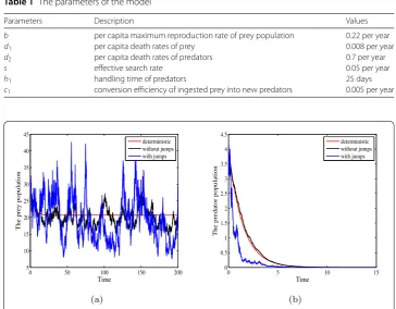
Figure 1Deterministic and stochastic trajectories of prey population and predator population with parameters in Table1. Moreover,σ2

1 =σ22= 0.005 andγ1(u) =γ2(u) = 0.05. (a) Trajectories of prey population.

(b) Trajectories of predator population. (Color figure online)

Thus,b– (d1+β1) = 0.2082, (

√

b–√d1+β1)2≈0.13 and _h1c1 –d2–β2< 0. Therefore, the conditions of Theorem 4.3are not satisfied while the condition of Theorem4.1is fulfilled. From Theorem4.1, it follows that the predator population becomes extinct with probability one. As can be seen from Fig.1that the prey population does not become extinct and predator population becomes extinct.

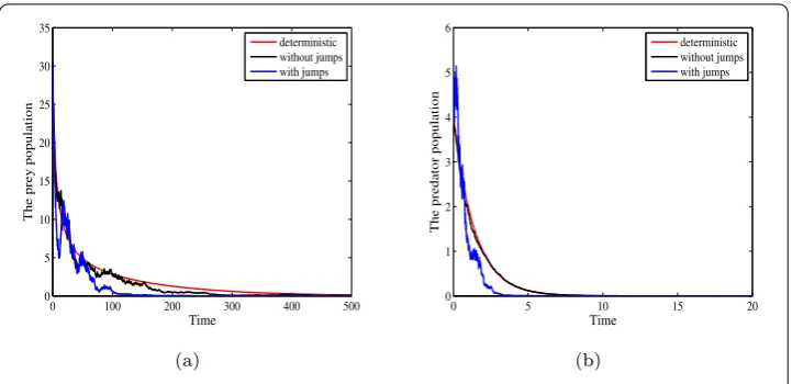
(ii) Moreover, for the sameα= 0.01, intensities of white noisesσ₁2=σ₂2= 0.005, jumps

γ1(u) =γ2(u) = 0.05 and greater Allee effect constant,A1= 20, we can obtainαA1= 0.2,

b– (d1+β1) = 0.2082 and (

√

b–√d1+β1)2= 0.1299. This implies the condition (ii) of Theorem4.3is fulfilled. Then, from Theorem4.3, it follows that both prey population and predator population become extinct. Figures2(a) and2(b) are the trajectories of prey population and predator population, respectively. From Fig.2, we can see that both prey population and predator population become extinct. Comparing Figs.1(a) and2(a), we can conclude that stronger Allee effects can lead to the extinction of the prey population, even if intensity of noise is not high.

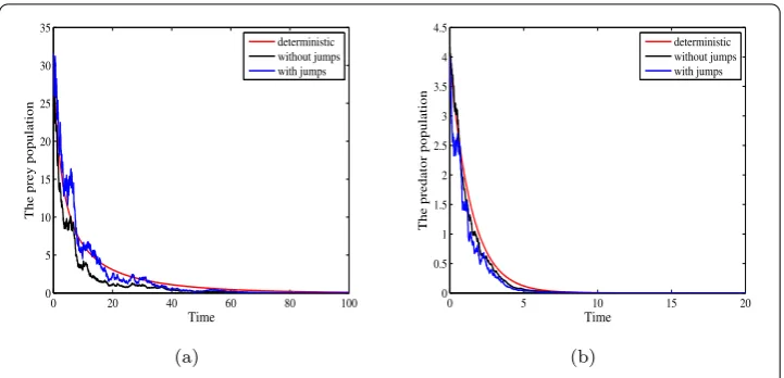
(iii) For the sameαandA1taken as those in (i). If intensities of white noisesσ12= 0.31,

σ₂2= 0.2 and jumpsγ1(u) = 0.1, γ2(u) = 0.05, thenαA1= 0.005,b– (d1+β1) = 0.0516, (√b–√d1+β1)2= 0.003481,b– (d1+

σ₁2

2) = 0.057 and (

√ b–

d1+

σ₁2

2 )

2_{= 0.00426. Then}

Figure 2Deterministic and stochastic trajectories of prey population and predator population with parameters in Table1. Moreover,α= 0.01,A1= 20σ12=σ22= 0.005 andγ1(u) =γ2(u) = 0.05. (a) Trajectories of

prey population. (b) Trajectories of predator population. (Color figure online)

Figure 3Deterministic and stochastic trajectories of prey population with parameters in Table1,α= 0.01,

A1= 0.5 and different intensities of white noise and jumps. (a)σ12= 0.31,σ22= 0.2,γ1(u) = 0.1,γ2(u) = 0.05.

(b)σ2

1= 0.05,σ22= 0.2,γ1(u) = 0.5,γ2(u) = 0.2. (Color figure online)

0.5,γ2(u) = 0.2, thenαA1= 0.005, b– (d1+β1) = 0.0165, (

√

b–√d1+β1)2= 0.00032,

b– (d1+

σ₁2

2 ) = 0.2095 and (

√ b–

d1+

σ₁2

2)

2_{= 0.1343. Thus, condition (ii) in Theorem4.3}

Figure 4Deterministic and stochastic trajectories of prey population and predator population withb= 0.02,

d1= 0.04,α= 0.01,A1= 3,σ12= 0.3,σ22= 0.2,γ1(u) =γ2(u) = 0.1 and other parameters are taken as in Table1.

(a) Trajectories of prey population. (b) Trajectories of predator population. (Color figure online)

then all conditions of Theorem 3.2 in [10] are not hold. From Fig.4, we can see that the prey population will become extinct with probability one and then the predator popula-tion.

7 Conclusions and discussions

In this paper, we consider a stochastic predator–prey population model with Allee effect and Lévy noise. First, by the comparison theorem of stochastic differential equations and the Itô formula, we prove that this model has a unique global positive solution starting from the positive initial value. Then we investigate the asymptotic pathwise behavior of the model by the generalized exponential martingale inequality and the Borel–Cantelli lemma. Next, we establish the conditions under which extinction of predator and prey populations occur. Furthermore, we show that the global positive solution is stochastically ultimate bounded under some conditions by using the Chebyshev’s inequality. At last, we introduce some numerical simulations to support the main results obtained.

Whenγ1(u) =γ2(u) = 0, we can get the stochastic predator–prey population (1.2), which is studied in [10]. From Remark 4.5, it follows that Corollary 4.4 generalizes and im-proves Theorem 3.2 in [10]. Moreover, our investigation shows that the Allee effect, white noise and jumps may cause great influence on the survival of species. It can be seen from Figs.1(a) and2(a) that stronger Allee effects can lead to the extinction of prey population, even if intensity of noise is not high. From Figs.1(a),3(a) and3(b), we can conclude that the high intensity noise and jumps can also lead to the extinction of prey population, even if the Allee effects is not large. Therefore, Allee effect is an important factor in population modeling. Moreover, considering the sudden environmental shocks, a stochastic model especially with jumps is better than a deterministic model in describing the population dynamics.

Funding

This work was supported by the National Natural Science Foundation of China (Nos. 11471197, 11571210, 11501339).

Availability of data and materials

Competing interests

The authors declare that they have no competing interests regarding the publication of this article.

Authors’ contributions

The study was carried out in collaboration with equal responsibility. All authors read and approved the final manuscript.

Publisher’s Note

Springer Nature remains neutral with regard to jurisdictional claims in published maps and institutional affiliations.

Received: 12 July 2018 Accepted: 26 February 2019

References

1. Freedman, H.I.: Deterministic Mathematical Models in Population Ecology. Dekker, New York (1980) 2. Pielou, E.C.: An Introduction to Mathematical Ecology. Wiley, New York (1969)

3. Kuussaari, M., Saccheri, I., Camara, M., Hanski, I.: Allee effect and population dynamics in the Glanville fritillary butterfly. Oikos82, 384–392 (1998)

4. Zu, J., Mimura, M.: The impact of Allee effect on a predator–prey system with Holling type II functional response. Appl. Math. Comput.217, 3542–3556 (2010)

5. Jiang, D., Shi, N., Zhao, Y.: Existence, uniqueness, and global stability of positive solutions to the food-limited population model with random perturbation. Math. Comput. Model.42, 651–658 (2005)

6. Liu, M., Bai, C.: Optimal harvesting of a stochastic logistic model with time delay. J. Nonlinear Sci.25, 277–289 (2015) 7. Takeuchi, Y., Du, N.H., Hieu, N.T., Sato, K.: Evolution of predator–prey systems described by a Lotka–Volterra equation

under random environment. J. Math. Anal. Appl.323, 938–957 (2006)

8. Lv, J., Wang, K.: A stochastic ratio-dependent predator–prey model under regime switching. J. Inequal. Appl.2011, 13 (2011)

9. Lian, B., Hu, S., Fan, Y.: Stochastic delay Lotka–Volterra model. J. Inequal. Appl.2011, Article ID 914270 (2011) 10. Jovanovi´c, M., Krsti´c, M.: Extinction in stochastic predator–prey population model with Allee effect on prey. Discrete

Contin. Dyn. Syst., Ser. B22, 2651–2667 (2017)

11. Zou, X., Wang, K.: Numerical simulations and modeling for stochastic biological systems with jumps. Commun. Nonlinear Sci. Numer. Simul.19, 1557–1568 (2014)

12. Applebaum, D.: Lévy Processes and Stochastic Calculus. Cambridge University Press, New York (2009)

13. Bao, J., Mao, X., Yin, G., Yuan, C.: Competitive Lotka–Volterra population dynamics with jumps. Nonlinear Anal.74, 6601–6616 (2011)

14. Bao, J., Yuan, C.: Stochastic population dynamics driven by Lévy noise. J. Math. Anal. Appl.391, 363–375 (2012) 15. Zhang, Q., Jiang, D., Zhao, Y., O’Regan, D.: Asymptotic behavior of a stochastic population model with Allee effect by

Lévy jumps. Nonlinear Anal. Hybrid Syst.24, 1–12 (2017)

16. Leng, X., Feng, T., Meng, X.: Stochastic inequalities and applications to dynamics analysis of a novel SIVS epidemic model with jumps. J. Inequal. Appl.2017, 138 (2017)

17. Peng, S., Zhu, X.: Necessary and sufficient condition for comparison theorem of 1-dimensional stochastic differential equations. Stoch. Process. Appl.116, 370–380 (2006)

18. Wu, R., Wang, K.: Population dynamical behaviors of stochastic logistic system with jumps. Turk. J. Math.38, 935–948 (2014)

19. Liu, Q., Chen, Q.M.: Asymptotic behavior of a stochastic non-autonomous predator–prey system with jumps. Appl. Math. Comput.271, 418–428 (2015)

20. Mao, X.: Stochastic Differential Equations and Applications. Horwood, Chichester (2007) 21. Lipster, R.: A strong law of large numbers for local martingales. Stochastics3, 217–228 (1980)