Complex System Maintainability Verification under Mixture Distribution

(1)

2019 International Conference on Artificial Intelligence and Computing Science (ICAICS 2019) ISBN: 978-1-60595-615-2

Complex System Maintainability Verification under Mixture Distribution

Zhen-ya WU* and Jian-ping HAO

Shijiazhuang Campus of Army Engineering University, Shijiazhuang, 050003, China *Corresponding author

Keywords: Complex system, Maintainability verification, Mean time to repair, Mixture distribution,

Hypothesis testing.

Abstract. Maintainability verification is an important work in system development. However, two problems arise when the maintenance time of complex system conforms to a mixture distribution. The first problem is the occurrence of assuming log-normal distribution instead of mixture distribution and the second one is the limited sample size for maintainability verification. Regarding the problems mentioned above, firstly, the maintenance sample generation process of complex system is analyzed and the mixture distribution model of maintenance time is proposed. Then, the changes in two types of test risks are analyzed when assuming log-normal distribution instead of mixture distribution. Finally, a method to perform maintainability verification using similar maintenance task’s samples is proposed. A case study using the maintenance time data of satellite communication interface system shows the efficiency of the proposed method.

Introduction

The goal of maintainability verification is to validate whether the maintainability metric (e.g., MTTR) satisfies consumer’s requirement. According to MIL-STD-471A, the test method for verification of MTTR are under the assumption that maintenance time can be adequately described by a log-normal distribution[1]. If no specific assumption concerns the distribution of maintenance time, the verification for MTTR can still be performed as the sample mean is approximately normal for large sample size by the central limit theorem.

In most cases, the log-normal distribution is the best model to be used to describe maintenance time distribution[2,3], while in special cases, the multi-modal distribution, which is also called mixture distribution, is sometimes a good representation for data samples with more than one factor of time dependency[4]. A random variable has a mixture distribution if its probability density function can be expressed by a convex combination of some probability density functions[5]. One of the first analyses involving the use of mixture distribution was undertaken by Karl Pearson which fitted a mixture of two normal probability density functions[6]. Since 1980s, many monographs studied the finite mixture distribution and its application mainly in clustering analysis[7-9].

During MTTR verification, it is usually difficult to obtain enough samples to perform goodness of fit analysis. Thus, the occurrence of assuming log-normal distribution for maintenance time when in fact it has mixture distribution might happen, especially for complex system. However, there are two problems still not completely clarified when the maintenance time of specified item has a mixture distribution:

(1) During the operational test and evaluation stage, it is difficult to obtain enough samples to check whether the maintenance time of the specified item conforms to a mixture distribution. The consequences when assuming log-normal distribution instead of mixture distribution remain to be researched.

(2) In a complex system, some maintenance tasks may show much similarities regarding repair actions, which makes their maintenance time probability density functions vary slightly. Thus, with the bearing of certain degrees of error, whether it is feasible to combine the samples from similar maintenance tasks in order to meet the sample size requirement is still a challenging problem.

(2)

time is proposed. In section 3, the error in producer’s and consumer’s risks when assuming log-normal distribution instead of mixture distribution and when combining samples from similar maintenance tasks are analyzed. Section 4 gives a case study using the maintenance records of satellite communication interface system to validate the proposed method. Finally, section 5 gives the conclusions of paper.

Mixture Distribution Model of Complex System Maintenance Time Basic Definitions of Mixture Distribution

Suppose that a random variable or vector,

X

, its distribution can be represented by a probability density function of the form

(1) where



_j 0, and

f_j()0



f_j(x)dx1 j1,,g

In such a case,

X

is said to has a finite mixture distribution and that

p

(



)

, defined by Eq. (1), is a finite mixture density function.

The parameters



₁,,



_g denote the mixing weights and f₁(),,f_g() denote the component densities of the mixture.

Maintenance Sample Generation Process Analysis of Complex System

As the major index to the character of maintainability, maintenance time is a function of design but affected by various personnel and logistic factors. Mixture distribution indicates that several distributions are present in the data. These distributions usually stem from different repair actions, different sets of maintenance personnel, maintenance instructions or different environments[10].

According to MIL-HDBK-505, item levels from the simplest division-‘part’, to the most complex division-‘system’, include subassembly, assembly, unit, group, set and subsystem[11]. For a complex system, it may have different types of failure modes due to its complex structure and composition. Thus, its corresponding maintenance tasks may have different time distribution functions caused by different repair actions.

Suppose a system has g types of maintenance tasks and their relative failure rates are



₁,,



_g(



₁



_g1).



T₁,,T_n



denotes a random maintenance time sample set of size

n

. Let

C_j denote a g-dimensional component-label vector, where the ith element of C_j, C_ij (C_j)_i, is defined to be one or zero, according to whether the sample T_j is from maintenance task

i

or not. Thus, C_j is distributed according to a multinomial distribution consisting of one draw on g

categories with probabilities



₁,,



_g; that is,

P(C_jc_j)



₁c1j



2 c2j



g

cgj ₍₂₎

Eq. (2) can also be written as:

(3)

Suppose that the conditional density of T_j given C_ij1 is f_i(t_j) which is the time probability density function of maintenance task

i

. Then, the unconditional density of T_j is given by p(t_j)

which has the

g

-component mixture form, that is:

(4) The mean and variance of T_j are[12]:

E[T_j]





i1 g





_i



_i (5)

E[(T_j



)2_]__d2_ i1

g





_i((



_i



)2__d i

2₎ ₍₆₎

where



_i and

d

_i are the mean and variance of time distribution function of maintenance task

i

.

MTTR Verification of Complex System

Assuming Log-Normal Distribution Instead of Mixture Distribution

Assume that the design goal maintainability index

H

₀ for the specified item is

MTTR





₀ and required maintainability index

H

₁ is

MTTR





₁. The producer’s risk is



and consumer’s risk is



.

According to MIL-STD-471A, if no specific assumption concerns the distribution of maintenance time, the sample size is given by:

(7)

where is a prior estimate of the variance of maintenance time.

If the maintenance time can be adequately described by a log-normal distribution, the sample size is given by:

(8)

where is a prior estimate of the variance of the logarithms of maintenance time. The decision criteria are:

Accept H₀, if X 



₀Z₁_ dˆ

n ; Reject H0, if X 



0Z1

ˆ

d

n (9)

where X is the sample mean, and

d

ˆ

is the sample standard deviation.

In the case of assuming log-normal distribution instead of mixture distribution, the producer’s risk is:

under H₀: P[X 



₀Z₁_ dˆ

n] (10)

(4)

P[X 



₀Z₁__ dˆ n]P[

X



₀

ˆ

d/ n 



₀Z₁__ dˆ n 



0

ˆ

d/ n ] P[

X 



₀

ˆ

d/ n z1]1 (z1)



The consumer’s risk is:

under

H

₁ : P[X 



₀Z₁_ dˆ

n] (11)

Eq. (11) can be written as:

P[X ₀Z₁__ dˆ n] P[

X₁ ˆ

d/ n 

₀Z₁__ dˆ n1

ˆ

d/ n ]

P[X 1 ˆ

d/ n Z1  n

ˆ

d (01)]

 [Z₁__  _ˆn

d (01)]

According to Eqs. (7) and (8), the sample sizes may be different between two distribution assumptions. Thus, the result indicates that, the producer’s risk will remain unchanged and consumer’s risk may have a change if log-normal distribution is assumed when in fact the maintenance time has a mixture distribution. Thus, during MTTR verification, it is important to check whether the maintenance time of specified item conforms to a log-normal distribution.

Combining Maintenance time Samples from Similar Maintenance Tasks

According to MIL-STD-471A, the test methods for MTTR verification all require a minimum or fixed sample size based on different distribution assumptions[1]. However, development budgets and schedules may not allow enough time to obtain the required number of maintenance tasks, especially for the equipment with high reliability.

For a complex system, there may be much similarities among some of its maintenance tasks, such as the maintenance tasks belonging to equipment which has almost same structure. These maintenance tasks may have time probability density functions with parameters varying a little. Thus, it might be a feasible method to combine their maintenance time samples for verification in order to meet the required sample size.

Suppose there are two maintenance tasks A and B, which show much similarities regarding their repair actions. They all conform to log-normal distribution with parameters varying a constant; that is:

lnT_A N(



_A,



_A2_{) ln}_T

B N(



Ag,



A

2 __h₎ ₍₁₂₎

and



_AeA 1 2A2

,d_A2__e2_A_A2

(eA21) ;



Be

(_Ag)1

2(A2h)

,d_B2 __e2(_Ag)(_A2__h₎

(e(_A2__h₎

1) (13) where g and h are constants.

Thus, if the maintenance time sample sets of task A and B are combined, it will conform to a mixture distribution; that is,

(5)



_A wA

w_Aw_B



B 

w_B

w_Aw_B (15)

where

w

_A and w_B are the failure rates of corresponding failure modes of task A and B. According to Eqs. (5) and (6), the mean



_AB and variance d_AB2 _are:



_AB



_A



_A



_B



_B (16)

d_AB2 _



A((



A



AB)

2__d

A

2₎_



B((



B



AB)

2__d

B

2₎ ₍₁₇₎

Assume that the design goal maintainability index for the combined data set is

H

₀

:



_AB





₀ and required maintainability index is

H

₁

:



_AB









.

If

H

₀ is true, according to Eqs. (13) and (16),



_A



_A₍_H

0)



B



B(H0) 



0



Ae

A(H_{0 )}

1 22A





_Be(A(H_{0 )}g)

1 2(2Ah)





₀





_A₍_H

0) ln



₀



_Ae

1 2A2





_Be

1 2(A2h)g

        (18) and

_A₍_H 0)e

A(H0 ) 1 2A2

,d_A₍_H 0) 2 __

A(H₀)

2 ₍_eA2 1) ;  B(H₀)e

(A(H0 )g) 1 2(A2h)

,d_B₍_H 0) 2 __

B(H₀)

2 ₍_e(A2h)1) (19)

and

d_AB₍_H

0)

2 _



A((



A(H₀)



0)

2_

d_A₍_H

0)

2

)



_B((



_B₍_H

0)



0)

2_

d_B₍_H

0)

2

) (20)

Thus, the distribution of X is:

X N(u_0,dAB(H0)

2

n_AB ) (21)

If

H

₁ is true, then



_A₍_H

1)ln



₁



_Ae

1 2A2





_Be

1 2(A2h)g

      

 (22)

and

_A₍_H

1)e

_A₍_H

1 ) 1 2A2

,d_A₍_H 1) 2 __

A(H1)

2 ₍_eA2 1) ; 

B(H1)e (_A₍_H

1 )g) 1 2(A2h)

,d_B₍_H 1) 2 __

B(H1) 2 ₍_e(_A2__h₎

1) (23) and

d_AB₍_H

1) 2 _



A((



A(H1)



1) 2__d

A(H1) 2 ₎_



B((



B(H1)



1) 2__d

B(H1)

2 ₎₍₂₄₎

(6)

X N(u_1,dAB(H1)

2

n_AB ) (25)

Then, under the asymptotic normality of

X

_n, n_AB can be defined as:

n_AB Z1dAB(H₀)Z1dAB(H₁)



₁



₀

      2 (26)

The sample size ratio of task A to B is same as the failure rate ratio; that is,

n

_A





_A

n

_AB

;

n

_B





_B

n

_AB (27) The decision criteria are:

Accept H₀, if X 



₀Z₁_ dˆ

n_AB ; Reject H0, if X 



0Z1

ˆ

d

n_AB (28)

If the test result of the combined data set is considered as the one of maintenance task A, the samples of task B may bring changes to the real test risks.

Assume that the real design goal maintainability index is H₀:



_A



₀ and required maintainability index is

H

₁

:



_A









.

If

H

₀ is true, then



_A₍_H

0)ln



0

1 2



A

2₍₂₉₎

and

_B₍_H 0)e

(_A₍_H 0 )g)

1 2(2Ah)

,d_A₍_H 0)

2 __ 0 2₍_e_A2

1) ; _AB₍_H

0)A0BB(H0),dB(H0)

2 __ B(H0)

2 ₍_e(_A2__h₎

1) (30) and

d_AB₍_H

0) 2 _



A((



0



AB(H0)) 2__d

A(H0) 2 ₎_



B((



B(H0)



AB(H0)) 2__d

B(H0)

2 ₎₍₃₁₎

the distribution of X is:

X N(



_AB₍_H

0),

d_AB₍_H

0)

2

n_AB ) (32)

Thus, the real producer’s risk is:



P[X 



₀Z₁_ dˆ

n_AB] (33)

If

H

₁ is true, then



_A₍_H

1)ln



1

1 2



A

2₍₃₄₎

and

_B₍_H 1)e

(A(H₁₎g)

1 2(A2h)

,d_A₍_H 1)

2 __ 1

2₍_e_A2

1) ; _AB₍_H

1)A1BB(H1),dB(H1)

2 __ B(H₁) 2 ₍_e(_A2__h₎

(7)

d_AB₍_H

1) 2 __

A((1AB(H1)) 2__d

A(H1) 2 ₎__

B((B(H1)AB(H1)) 2__d

B(H1)

2 ₎₍₃₆₎

the distribution of X is:

X N(



_AB₍_H

1),

d_AB₍_H

1)

2

n_AB ) (37)

Thus, the real consumer’s risk is:



 P[X 



₀Z₁_ dˆ

n_AB] (38)

Case Study

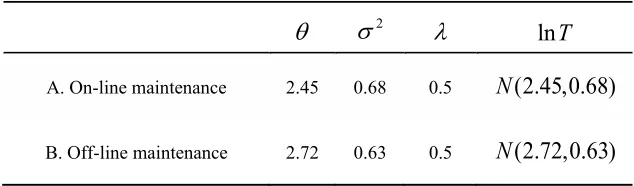
[image:7.612.147.464.336.429.2]

In this section, two sets of maintenance time samples from Defense Communication System/Satellite Control Facility Interface System (DSIS) Maintainability Demonstration Report are combined for MTTR verification. The equipment has much redundancy which allows on-line maintenance by “reconfiguration” the system by patching[13]. Table 1 shows the probability density functions of the two data sets[2].

Table 1. Maintenance time probability density functions of DSIS.





2



ln

T

A. On-line maintenance 2.45 0.68 0.5

N

(2.45,0.68)

B. Off-line maintenance 2.72 0.63 0.5

N

(2.72,0.63)

Assume that the design goal maintainability index

H

₀ for the combined data set is



_AB



15min

and required maintainability index

H

₁ is



_AB



20min

and the producer’s and consumer’s risks are









0.05

.

According to Eq.(26), the required sample size is:

n_AB 1.6514.561.6519.42 2015

 

 

2

125.7126

and the required sample size for maintenance task A and B are:n_An_B 0.512663

In fact, the real specified item is the on-line maintenance task. Thus, the design goal maintainability index

H

₀ is



_A



15min

and required maintainability index

H

₁ is



_A20min and the producer’s and consumer’s risks are









0.05

.

If

H

₀ is true, according to Eqs. (29) ~ (32), the distribution of sample mean is:

X  N(17.08,2.18) Thus, according to Eq. (33), the real producer’s risk is:



P(X 151.65212.09

126 )0.48

(8)

X N(22.78,3.89) Thus, according to Eq. (38), the real consumer’s risk is:



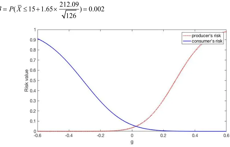
 P(X 151.65212.09 [image:8.612.99.472.110.348.2]

126 )0.002

Figure 1. The relationship between

g

and risk values(

h

 

0.05

).

Figure 2. The relationship between

h

and risk values(g0.27).

The above results indicate that if the two maintenance time sample sets are combined for MTTR verification of on-line maintenance task, the real producer’s risk increases the number of about 0.43 while consumer’s risk decreases the number of about 0.048. It means that it is difficult to accept the equipment if it doesn’t meet the requirement but easy to reject it for not meeting the requirement when, in fact, it has. Thus, during MTTR verification, if the equipment is rejected for the hypothesis test, further investigation need to be made to confirm whether it is acceptable. Fig. 1 and Fig. 2 show the risk values with different values of g and h.

[image:8.612.138.473.381.578.2]

(9)

n_A



Z



0Z



1



2



₁



₀





2 (e

2A1) (1.65151.6520)

2

(2015)2 (e

0.68_₁₎__129.9_₁₃₀

Thus, nearly half the number of sample size can be saved if on-line and off-line maintenance sample sets are combined for maintainability verification.

Conclusions

Maintenance time of complex system sometimes conforms to mixture distribution due to its various maintenance tasks. During maintainability demonstration, as it is difficult to perform goodness of fit analysis with the limited sample size, there will be error in test risks caused in assuming log-normal distribution when in fact it has mixture distribution. On the other hand, for the maintenance tasks of complex system, there may be much similarities between some of them. Thus, the samples of similar maintenance tasks can be used as a supplement to the specified task’s samples to implement maintainability verification.

Regarding the issues mentioned above, firstly, the maintenance sample generation process of complex system was analyzed and the mixture distribution model of maintenance time was proposed. Then, this paper analyzed the changes in two types of test risks when assuming log-normal distribution instead of mixture distribution. Finally, a method to perform maintainability verification using maintenance time data from similar maintenance task was proposed. A case study using the maintenance time data of satellite communication interface system was presented as an example of the proposed method.

References

[1] MIL-STD-471A. Maintainability verification/demonstration/evaluation, 1975.

[2] R. Almog, A study of the application of the lognormal distribution to corrective maintenance repair times, M.S. thesis, Naval Postgraduate School, 1979.

[3] E. Camozu, A Study of the application of the lognormal and gamma distribution to corrective maintenance repair time data.

[4] IEC 60706-3 Maintainability of equipment-Part 3: Verification and collection, analysis and presentation of data, 2006.

[5] D.M. Titterington, A.F.M. Smith, U.E. Makov, Statistical Analysis of Finite Mixture Distributions, John Wiley & Sons, Chichester, 1985.

[6] K. Pearson, Contributions to the theory of the mathematical evolution, Philosophical Transactions of the Royal Society of London. A(185) (1984) 71-110.

[7] B.S. Everitt, D.J. Hand, Finite Mixture Distributions, Chapman & Hall, London, 1981.

[8] G.J. McLachlan, K.E. Basford, Mixture models: Inference and applications to clustering, Statistics Textbooks & Monographs New York Dekker. 38(2) (1988).

[9] G.J. McLachlan, D. Peel, Finite Mixture Models, John Wiley & Sons, New York, 2000. [10]David J. Smith, Alex H. Babb, Maintainability Engineering, Pitman, Bath, 1973.

[11]MIL-HDBK-505. Handbook for definitions of item levels, item exchangeability, models, and related terms, 1998.

[12]Sylvia Frühwirth-Schnatter, Finite Mixture and Markov Switching Models, Springer, New York, 2006.