Fast Straight Line Detection Method Based on Directional Coding

2019 International Conference on Computer Science, Communications and Big Data (CSCBD 2019) ISBN: 978-1-60595-626-8

Fast Straight Line Detection Method Based on Directional Coding

Su-Yun LUO

, Zhi-Yong TANG and Xu WANG

School of Mechanical and Automotive Engineering, Shanghai University of Engineering Science, Shanghai, China

*Corresponding author

Keywords: Directional coding, Hough transform, Line detection.

Abstract. The Standard Hough Transform (SHT) is robust in detecting dashed or broken lines, but the main parts of it, blind vote, can cause excessive consumption of computation. To overcome this disadvantage, a fast straight line detection method based on directional coding(DCHT) is described in this paper. The algorithm turns the exhausted task of voting for all directions into an elegant task by constructing a sniffer and predicting direction of straight lines around the pixels. By using directional coding approach, the algorithm proposed here treats each direction of edge pixels differently, voting for a smaller angle range covering the direction of straight line which contains this edge pixel. In this way, half or more voting is removed. Experimental results show that DCHT algorithm has significant performance in reducing both execution time and the influence of noise on parameter space.

Introduction

Straight line detection comprising issues such as vanishing point detection, line matching across views and parallel line detection, is a fundamental research field in computer vision. Hough Transform(HT) and Standard Hough transform(SHT) [1] is the primary solution to straight line detection and is widely used because of its robustness for detecting discontinuous lines.

Although SHT is a well-known algorithm, it still has some disadvantages which can’t be ignored. Many scholars have carried out thorough research on them and put forward improved algorithms. Such as, inaccurate parameterization may result in process noise or model noise but can be remedy by using suitable parameterization and mapping[2], uniform quantization may result in reduced precision of curve detection but can be remedy by using several methods such as subunity quantization step for the intercept[3], diagonal quantization technique[4], non-uniform quantization[5], etc. In blind voting, each pixel contributes equally for a feature detection, which is time consuming. The paper of Qiang[6] proposed a probabilistic scheme which analytically estimated the uncertainty of the line parameters derived from each feature point, based on which a Bayesian accumulator updating scheme was used to compute the contribution of the point to the accumulator.

This paper aims to reduce the blindness of traditional HT in the voting process. Traditional methods take the angle in the range of 180 degrees for each edge pixel into consider, while the proposed method here only consider the angle in the range of 90 degrees or even 45 degrees. As we know, the more information about the direction of straight line through the pixel we know, the more we can reduce the blindness of voting by limiting the range of angles. However, the pursuit of more information requires a greater computation and more time consumption. The method proposed in this paper can obtain enough information through a simple algorithm mand reduce the computation and time needed greatly.

Directional Coding Hough Transform (DCHT)

Terms

Terms used in this paper are explained here.

Pattern of pixel P: pixel P is defined as the central pixel which is the shadow region in Figure 1-a. Pattern of pixel P is defined as the distribution of P’s neighborhood values in space. Figure 1-b shows a pattern. For convenience, set an identifier for each position(from 0 to 7), shown in Figure 1-a. There are 256 patterns in total;

(a) Neighborhood with identifiers (b) A case of pattern

Figure 1. Pattern of pixel.

Figure 2. Defined 4 basis direction. Figure 3. Primitives in 8 directions.

i

n : value in position i; SP Numeric String(NS) of central pixel P. In this paper, NS has two

forms. 8-digit form, SP 'n n0 1 n7'. 4-digit form, SP '(n0n4) ( n1n5) ( n2n6)(n3n7) '.

The symbol “∙” here is used as a partition;

P

SS : sum of NS S_P, SS_P 



if SP'11010010', then SPnZ{1}0,SPnZ{2} 1, SPnZ{3} 3, SPnZ{4}6;

i: diagonal position of position i, i  i 4. The addition and subtraction of identifier in this paper is octal. The essence of this operation is to obtain the diagonal position in Figure 1-a;

i j : included angle of basis directions cross over position i and j. Four basis directions are defined (shown in Figure 2 as angle 45°, 0°, −45°, −90°) In this paper, the angle range is [−90°, 90°).

Restricted Pattern Analysis and Direction Prediction

Section 2.2, all the discussions are under this assumption and the "restricted" in section headline refers to this.

It is easy to verify that each pixel P except the endpoints belongs to a straight line which conforms to the Freeman norm can satisfy the following expressions:

2

SS



(1)

{1} {2}

|

S



S

| {0,1}



Direction Prediction. For the pixel P on a straight line satisfying the Freeman norm, except endpoints, we make the following assertions.

1) If |S_PnZ{1}S_PnZ{2}| 1 , we predict the direction of the straight line which pixel P belongs is

within the angle S_PnZ{1}S_PnZ{2}.

2) If |S_PnZ{1}S_PnZ{2}| 0 , the direction is predicted within the angle (SPnZ{1} 1) (SPnZ{1}1).

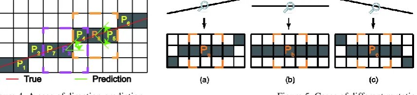
The assertions were explained as following: We interpret Freeman norm as the ‘reconciliation’ of two adjacent primitives’ directions and the ‘frequency’ of the chain code’s appearance represents the ‘extent’ of that the real direction of straight line approaches code’s corresponding direction. Typically, when two chain codes appear at the same frequency, it means that the true direction of the straight line is in the middle of their corresponding direction. Since the pattern is local information, the frequency of the chain code cannot be provided, so the angle range of the true direction can only be inferred by pattern. The object described by chain codes is line while the object described by NS is pattern. According to Eq. 2, all pixels except the endpoints are divided into two classes. As shown in Figure 4, pixels such as𝑃₁, 𝑃₂, 𝑃₃, 𝑃₄, 𝑃₅, 𝑃₆ which satisfy |𝑆_{𝑃𝑛𝑧{1}}− 𝑆𝑃𝑛𝑧{2}−| = 1 are classified as mutation class while the other pixels, for example𝑃7, 𝑃8, are

classified as constant class. Mutation class means two chain codes appear while constant class means only one chain code appear nearby. For pixels belonging to mutation class, we reckon that the true direction of the line is a ‘reconciliation’ version of two basis directions. Take 𝑃₃ as an example, the two nonzero positions are ‘1’ and ‘4’ and their corresponding basis directions are 45° and −90°. So we predict that the direction of 𝑃₃ is within (45°, 90°) (90° and − 90°) are refer to same basis direction and this can be easy verified by case shown in Figure 4. For pixels belonging to constant class, it is difficult to ensure that ‘mutation’ occurs in a limited area. Such as the three cases shown in Figure 5, for pixels 𝑃_𝑎, 𝑃_𝑏, 𝑃_𝑐, although chain code of the current region remains consistent, after an indefinite length of distance, case in (a) has an anti-clockwise ‘mutation’, case in (c) has a clockwise mutation and case in (b) has no mutation. So we adapt to all possible scenarios by expanding the angle of prediction. The case of 𝑃8 in Figure 4 shows the

angle more intuitively.

Figure 4. A case of direction prediction. Figure 5. Cases of different mutation.

Pattern Analysis and Direction Prediction. For the patterns in 8-neighborhood, there are 28 _{= 256 variants. Calculate the sum 𝑆𝑆}

𝑃, for each pattern’s NS separately and then discuss them

1) 𝑆𝑆𝑃 ≤ 1. Patterns in this case do not provide sufficient information to indicate that its

central pixel belongs to any straight line. So we recommend to ignore the pixels whose pattern belongs to this case during voting process.

2) 𝑆𝑆𝑃 = 2. For pixels on a fine line, most of their patterns should fall into this category. So we

use Eq. 2. to sniffer the pattern whose central pixel may belong to a straight line. And then use the assertions to make a prediction. For those central pixels whose pattern does not satisfy Eq. 2, we also abandon them in voting procedure.

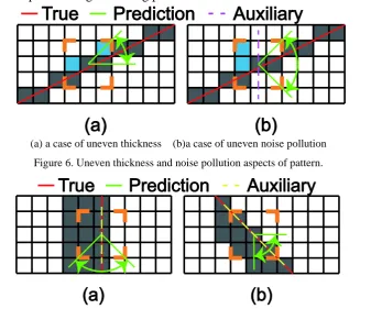
3) 𝑆𝑆𝑃 ∈ {3,4}. In this case, the patterns are discussed in two aspects: uneven thickness and

noise pollution. Most of the previously mentioned lines in this paper need to satisfy the fine line assumption. However, after revise the pattern, lines are allowed to be slightly uneven in thickness. Method applied here can be described as deleting one of the diagonal positions and evaluating the modified pattern by Eq. 1 and Eq. 2. If these two equations are satisfied, we consider that this pattern may belong to the pixel on a straight line where the thickness is uneven and then assertions are used for making a prediction (shown in Figure 6).

4) 𝑆𝑆𝑃 = 5. We reckon these cases similar to those whose half sides are filled, shown in Figure

7. The pixel on the edge of the thick straight lines may have this form of pattern and we consider it motivated by improved program robustness. This form of pattern can be picked out by identifying whether there are 5 consecutive nonzero values in its NS or not.

5) 𝑆𝑆_𝑃 ≥ 6. In this case, the pattern can’t provide sufficient information to indicate that the central pixel belongs to a straight line because of serious noise pollution. So we recommend ignoring their central pixel during the voting process.

(a) a case of uneven thickness (b)a case of uneven noise pollution

Figure 6. Uneven thickness and noise pollution aspects of pattern.

Figure 7. Cases of thick straight lines.

The pattern is not a sufficient condition to conclude that if the pixel with this pattern belongs to a straight line or not. Here may be a mistake to make a prediction for the pixels that don't belong to any straight line. But as long as the pixel is on a fine line, its pattern can certainly be picked up and used for making prediction.

Pattern Encoding and Simplifying

is to find a better form of NS which can beeasily processed. The other is to reduce the number of patterns.

Pattern Convolution Encoding. NS is propitious tomaking conclusion but it would be more convenient for algorithm programming if it was converted to convolution. Typically, we can get the corresponding convolution result of a NS by setting the kernel as following:

𝐾 = [10

4 ₁₀5 ₁₀6

103 _{0 10}7

102 _{10 1}

]

The essence of convolution operations here is to map different patterns to different positions on the real axis. This mapping is reversible, so we can also analyze patterns and predict directions using the convolution.

Pattern Simplifying. Because diagonal position scrossed by same basis direction, the same direction information is expressed. Take the patterns shown in Figure 8 as an example, the patterns of A and B are different. However, they can obtain the same predicted direction of straight lines because their nonzero position sare diagonal. If they can be merged by a unified expression, then the number of patterns can be reduced. If we merge the values of diagonal positions we then get a new shorter NS with only4-digit. For instance, as shown in Figure 8, when merged NS ‘01001000’ and ‘10000100’, we got NS ‘1100’. In convolution operations, this can be achieved by setting the diagonal weights of the kernel equation.

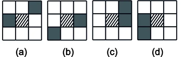
After merging the patterns, strategy mentioned in Section 2.3 needs to be fixed and it will be listed later in the form of specific convolution kernel. In addition, one thing need to be note is the merged form inevitably introduces some noisy pattern because of the confusing of the diagonal positions. For better illustration, an example is given in Figure 9. All four patterns shown in the figure have a unified form ‘1100’, but only two patterns, that’s (a) and (b), satisfy the Eq. 2. Therefore, in fact only patterns (a) and (b) should be used to make predictions. However, by the unified form we can’t distinguish (a), (b), (c) and (d), thus, noise is introduced. Fortunately, these noise only cause a little extra calculation.

Figure 8. Example of diagonally positions with the same direction information.

Figure 9. Four patterns of the same unified form ‘1100’.

𝐾 = [

𝑞 𝑝 𝑛 𝑚 0 𝑚

𝑛 𝑝 𝑞] m < 𝑛 < 𝑝 < 𝑞 ; 𝑚, 𝑛, 𝑝, 𝑞 ∈ 𝑁+ ; (3)

n ≠ 2 ∙ m ; (4)

p ≠ x ∙ m + y ∙ n ; x, y ∈ {0, 0.5, 1, 2} ; (5)

q ≠ x ∙ m + y ∙ n + z ∙ p ; x, y, z ∈ {0, 0.5, 1, 2} ; (6) The kernel used in this paper is:

𝐾 = [10

3 ₁₀2 ₁₀

1 0 1

10 102 ₁₀3

]

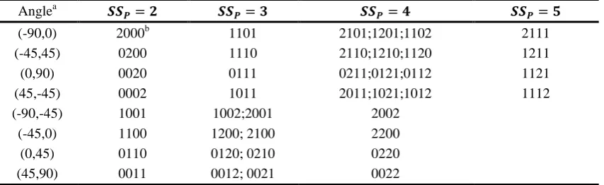
Combining the analysis mentioned in Section 2.3 with the specific kernel, we obtain the corresponding relation between the patterns expressed by convolution results and the predicted direction, shown in Table 1.

Table 1. Strategy details for predicting direction.

Anglea 𝑺𝑺𝑷= 𝟐 𝑺𝑺𝑷= 𝟑 𝑺𝑺𝑷 = 𝟒 𝑺𝑺𝑷= 𝟓

(-90,0) 2000b 1101 2101;1201;1102 2111 (-45,45) 0200 1110 2110;1210;1120 1211 (0,90) 0020 0111 0211;0121;0112 1121 (45,-45) 0002 1011 2011;1021;1012 1112 (-90,-45) 1001 1002;2001 2002

(-45,0) 1100 1200; 2100 2200 (0,45) 0110 0120; 0210 0220 (45,90) 0011 0012; 0021 0022

a

Refer to angles defined in Figure 2;

b

Result of convolution presented in4-digit tobetter correspond to its unified form

Experiment

Configuration and Preparation

In this article, three straight line detect algorithms, Standard Hough Transform (SHT), Progressive Probabilistic Hough Transform (PPHT) and the proposed algorithm DCHT, were implemented.

Experiments were done on a set of images which contain lanes, buildings, and synthetic straight lines. Because of the fact that there are too many lines in the real image, it’s impossible to list exhaustively. In order to evaluate the performance of these algorithms, straight lines making the contours of lane lines, main structural components of buildings or any other conspicuous lines were selected by human experts and were stored as ground truth.

Comparison of Detection Rate

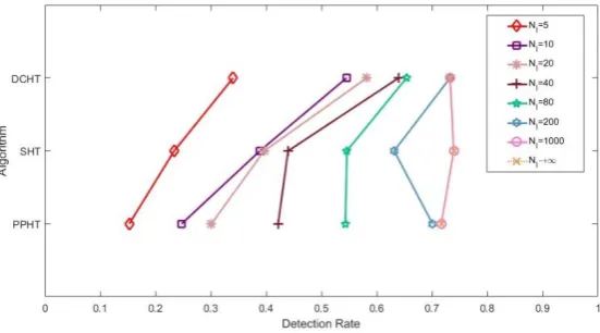
The detection rate in this paper is defined as the percentage of correctly detected ground truth under some user-defined parameters. In order to visually analyze the effect of the maximum number of straight lines 𝑁_𝑙 on the detection rate, detection rate results are shown in Figure 10, with 𝑁_𝑙 set to 5, 10, 20, 40, 80, 200, 1000 and ∞(𝑁_𝑙 is a parameter defined in algorithm programming, the program will stop detecting straight line when the number of straight line detected reaching 𝑁𝑙). It

should be note that the detection rate when𝑁𝑙 equals ∞is not calculated but manually set as the

convergent detection rate.

detection rate of PPHT is the lowest. The difference between the highest and the lowest is nearly doubled. Because of applying directional coding technique to filter parts of the voting, with DCHT algorithm not only the blindness voting is reduced but also the background noise is suppressed. So finding more straight lines is exposed. By using random sampling technique, it is difficult for the PPHT algorithm to extract straight lines from a large amount of noise due to the limitation of local information while SHT and DCHT extract the lines at the end of voting can make full use of global information. With the increasing of 𝑁_𝑙, DCHT converges to a value earlier than the other two algorithms. SHT and PPHT will converge respectively to a value which is approximately equal to that of DCHT in the end. This is may be because of the reason that greater 𝑁𝑙 exhausts all possible

positions of the straight lines.

Figure 10. Detection rate of three algorithms with different 𝑁𝑙.

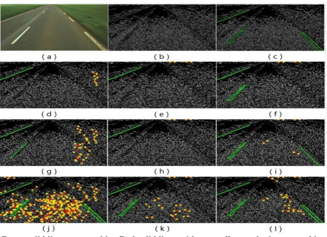
Green solid lines: correct hits, Red solid lines with two yellow endpoints: error hits

(a), (b), (c): Original image, its edge image and image with ground truth, Green solid lines denote ground truth (d), (g), (j): Results of PPHT with 𝑁𝑙 set to 5, 20, 200 respectively

(e), (h), (k): Results of SHT with 𝑁_𝑙 set to 5, 20, 200 respectively (f), (i), (l): Results of DCHT with 𝑁𝑙 set to 5, 20, 200 respectively

Figure 11. Comparison of algorithm results on road image.

The parameter spaces of SHT and DCHT are given in Figure 12. As we can see the voting number of DCHT is only about half of SHT. In addition, it can be clearly seen that the reduction in overall voting highlights the straight lines and make them easier to be detected.

The above example is not a coincidence. Several examples are given here. Results on house image are shown in Figure 13 while results on room image are shown in Figure 14. It should be noted that in these two examples, 𝑁_𝑙 is set to 40. These two examples are somewhat different from the previous one because of the perceptually reasonable straight lines. The walls of the house and the floor of the room are accompanied by a lot of different shades. It can be seen from these figures that, DCHT and SHT have less false detection compared to PPHT, and DCHT can usually hit more ground truth than SHT. In conclusion, DCHT can give a more satisfactory result than SHT and PPHT in straight line detection.

(a) Parameter space of SHT (b) Parameter space of DCHT

(a) Original image; (b) Edge image ; (c) Results of PPHT with 𝑁𝑙= 40; (d) Results of SHT with 𝑁𝑙= 40; (e) Results

of DCHT with 𝑁𝑙= 40

Figure 13. Results on house image.

(a) Original image ; (b) Edge image ; (c) Results of PPHT with 𝑁𝑙= 40; (d) Results of SHT with 𝑁𝑙= 40; (e) Results

of DCHT with 𝑁𝑙= 40

Figure 14. Results on room image.

Comparisons of Execution Time

Algorithm efficiency measuring requires collecting the times that algorithmscost. The execution time includes the time of edge detection, Hough voting procedure as well as peaks and lines extraction. In the extraction phase, the time consuming of PPHT is zero because its extraction operation is interspersed with the voting process while the other two algorithms implemented by calling MATLAB’s built-in function. The results are shown in Figure 15.

By analyzing the results shown in Figure 15, It can be figured outthat compared with SHT, the time consumption of DCHT is reduced by half, but slightly higher than PPHT. As to the edge detection stage, a same algorithm canny was applied in the programs of the three algorithms so their time consumptions at this stage are equal. In the voting process, DCHT and PPHT have less time consuming than SHT. In order to get the comparison of the algorithms, in the test of PPHT we set 𝑁_𝑙→ ∞. It means PPHT would exhaust all the edge points and cost more time. But in general algorithms procedures stop while a predetermined number of lines are detected, which consumes less time than that of the algorithm shown in Figure 15. And this is indeed the advantage of using stochastic method. In the process of peaks and lines extraction, SHT and DCHT called the function provided by MATLAB and we can see DCHT consumes less time than SHT.

Summary

In this paper, a fast line detection method based on directional coding is given. This algorithm is improved based on SHT. Using the directional coding technique, a sniffer is designed to predict the direction of the straight line and to vote selectively within a small angle. Experimental results show that the algorithm presented in this article not only has superior detection rate but also is time saving compared to SHT. In addition, in principle, the core of the directional coding algorithm, can be used along with other algorithms and can promote each other. Since the algorithm is improved both in execution time and noise suppression, it is very suitable for applications which requires both speediness and efficiency such as lane lines detection.

References

[1] PVC Hough, Method and means for recognizing complex patterns[P], USA, U.S. Patent, no.3069654, 1962.

[2] Mukhopadhyay P, Chaudhuri B B. A survey of Hough Transform[J]. Pattern Recognition, 2015, 48(3):993-1010.

[3] Ioannou D, Dugan E T. A note on “A fresh look at the Hough transform” [M]. Elsevier Science Inc. 1998.

[4] Leung D N K, Lam L T S, Lam W C Y. Diagonal quantization for the Hough transform[J]. Pattern Recognition Letters, 1993, 14(3):181-189.

[5] Duan H, Liu X, Liu H. A Non-uniform Quantization of Hough Space for the Detection of Straight Line Segments[C]//International Conference on Pervasive Computing and Applications. IEEE, 2007:149-153.