A hybrid splitting method for smoothing Tikhonov regularization problem

(1)

R E S E A R C H

Open Access

A hybrid splitting method for smoothing

Tikhonov regularization problem

Yu-Hua Zeng

1,2

_{, Zheng Peng}

3

_{and Yu-Fei Yang}

1*

*_{Correspondence:}

[email protected]

1_{College of Mathematics and}

Econometrics, Hunan University, Changsha, 410082, China Full list of author information is available at the end of the article

Abstract

In this paper, a hybrid splitting method is proposed for solving a smoothing Tikhonov regularization problem. At each iteration, the proposed method solves three

subproblems. First of all, two subproblems are solved in a parallel fashion, and the multiplier associated to these two block variables is updated in a rapid sequence. Then the third subproblem is solved in the sense of an alternative fashion with the former two subproblems. Finally, the multiplier associated to the last two block variables is updated. Global convergence of the proposed method is proven under some suitable conditions. Some numerical experiments on the discrete ill-posed problems (DIPPs) show the validity and eﬃciency of the proposed hybrid splitting method.

Keywords: Tikhonov regularization; augmented Lagrangian method; parallel splitting method; alternative direction method of multipliers

1 Introduction

In this paper, we consider a smoothing Tikhonov regularization problem, which is an un-constrained minimization of the form []

minAx–b+δx+ηxp_p, (.)

whereA∈Rm×n,b∈Rm, andx∈X⊂Rn, and · denotes the Euclid norm. The param-etersδ≥ andη≥ are used to control the smoothness and size of the approximate solution. Matrixis a (tridiagonal, Toeplitz) matrix,xrepresents a measure of the vari-ation or smoothness ofx, where

=n ⎛ ⎜ ⎜ ⎜ ⎜ ⎜ ⎜ ⎜ ⎜ ⎜ ⎜ ⎜ ⎝

 –   · · ·    

  –  · · ·    

   – · · ·    

..

. ... ... ... ... ... ... ...

    · · · –   

    · · ·  –  

    · · ·   – 

⎞ ⎟ ⎟ ⎟ ⎟ ⎟ ⎟ ⎟ ⎟ ⎟ ⎟ ⎟ ⎠

∈R(n–)×n. (.)

The smoothing regularization problem (.) has numerous applications in many ﬁelds, in-cluding mathematical programs with vanishing constraints [], maximum-likelihood es-timation problem [], language modeling [], and so on.

(2)

The last term of the problem (.),ηxpp, is a regularization term. As a common

reg-ularization method,regularization (p= ) problem has many good properties since it is a convex programming problem. In recent years, there has been an increasing inter-est in theregularizer. Theregularization model can reconstruct the original signal with less observed signals, when the original signal is spare or the observed signal contains noise. Especially, theformulation suits signiﬁcantly better for denoising data containing so-called outliers,i.e., observations containing large measurement errors []. Therefore, mathematical models and large-scale fast algorithms associated withregularization can be seen everywhere in compressed sensing, signal/image processing, machine learning, statistics, and many other ﬁelds [–].

Byregularization, the problem (.) reduces to

minAx–b_+δx_+ηx. (.)

It is identical to a separable convex minimization of the form

⎧ ⎪ ⎨ ⎪ ⎩

min

Ax–b ₊

δy ₊_η_z

, s.t.x–y= ,

y–z= .

(.)

The augmented Lagrangian function associated to the problem (.) is

L(x,y,λ,z,μ) = 

Ax–b ₊

δy

_–_λT₍_x_–_y_{) +}β

x–y 

–μT(y–z) +ηz+

ρ

y–z

_. _(.)

Indeed, there are many methods for solving the problem (.) in the literature. Among these methods, the parallel splitting augmented Lagrangian method and the alternating direction method of multipliers are two power tools. The recent research indicates that, due to the separable convex optimization with three block variables, the direct extension of the alternating direction method of multipliers is not necessarily convergent []. Thus, some hybrid splitting methods can be found in the literature. For example, see He [], Peng and Wu [], and Glowinski and Le Tallec [].

The saddle point of a Lagrange function associated to the convex optimization problem (.),w∗= (x∗,y∗,λ∗,z∗,μ∗)∈W, satisﬁes the following variational inequalities:

⎧ ⎪ ⎪ ⎪ ⎪ ⎪ ⎪ ⎨ ⎪ ⎪ ⎪ ⎪ ⎪ ⎪ ⎩

(x–x∗)T[AT(Ax∗–b) –λ∗]≥, (y–y∗)T_[_δT_y∗₊_λ∗_–_μ∗_]_≥_,

(λ–λ∗)T₍_x∗_–_y∗₎_≥_,

ηz–ηz∗+ (z–z∗)T[μ∗]≥, (μ–μ∗)T₍_y∗_–_z∗₎_≥_,

∀w=x,y,λ,z,μ∈W, (.)

where

W=X×X×Rn×X×Rn⊂R×n.

(3)

pro-posed method, referred to as the hybrid splitting method (HSM), will combine a parallel splitting (augmented Lagrangian) method and an alternating directions method of mul-tipliers. In the HSM, the predictor of the new iterate,w˜k_{= (}_x_˜k_,_y_˜k_,_λ˜k_,_z_˜k_,_μ_˜k_{), is got in the}

following way: ﬁnd (x˜k,y˜k) in a parallel manner, and updateλ˜k. Then computez˜k alter-nately with (x˜k_,_y_˜k_{), and update}_μ_˜k _{at the last. The new iterate is produced by a correct}

operator. The global convergence of the HSM is proven under some wild assumptions. The rest of this paper is organized as follows. In Section , we describe the proposed hybrid splitting method. Section  is devoted to showing that the sequence{wk}generated by the HSM is Fejér monotone with respect to the solution set. Then, the convergence of the HSM is proved. In Section , some preliminary numerical results are presented which indicate the feasibility and eﬃciency of the proposed method. Finally, some concluding remarks are made in Section .

2 The hybrid splitting method

In this section, we ﬁrst propose a hybrid splitting method for the problem (.), and then we give some remarks on the described method.

Algorithm .(The hybrid splitting method (HSM)) For a givenwk_{= (}_xk_,_yk_,_λk_,_zk_,_uk₎_∈ W,βk> , andρk> , the HSM produces the new iteratewk+= (xk+,yk+,λk+,zk+,uk+)∈ Wby the following scheme:

S. Producew˜k_{= (}_x_˜k_,_y_˜k_,_λ˜k_,_z_˜k_,_μ_˜k₎_{by s. to s..}

s.. Findx˜k_∈_X _{(with ﬁxed}_yk_,_λk_,_zk_,_μk_,_β

k,ρk) such that

x–x˜kATA˜xk–b–λk+βk

˜

xk–yk≥, ∀x∈X. (.)

s.. Findy˜k_∈_X_{(with ﬁxed}_xk_,_λk_,_zk_,_μk_,_β

k,ρk) such that

y–y˜kδTy˜k+λk–μk–βk

xk–y˜k+ρk

˜

yk–zk≥, ∀y∈X. (.)

s.. Updateλ˜kvia

˜

λk=λk–βk

˜

xk–y˜k. (.)

s.. Findz˜k_∈_X _{(with ﬁxed}_x_˜k_,_y_˜k_,_λ˜k_,_μk_,_β

k,ρk) such that

ηz_–ηz˜k_+z–z˜kμk–ρk

˜

yk–˜zk≥, ∀z∈X. (.)

s.. Updateμ˜kvia

˜

μk=μk–ρk

˜

yk–˜zk. (.)

S. Convergence veriﬁcation: for a given smallε> , ifwk–w˜k∞<εthen stop, and acceptwk_{to be the approximate solution. Else, go to S.}

S. Produce the new iterate by

wk+=wk–αkd

(4)

where

αk=γ αk∗, γ∈(, ), (.)

α_k∗= ϕ(w

k_,_w_˜k₎

d(wk_,_w_˜k₎

G

, (.)

and

ϕwk,w˜k=wk–w˜k_G, dwk,w˜k=Mwk–w˜k, (.)

G= ⎛ ⎜ ⎜ ⎜ ⎜ ⎜ ⎜ ⎝ βk     

 βk+ρk

   

  _β

k  

   ρk

 

    _ρ

k ⎞ ⎟ ⎟ ⎟ ⎟ ⎟ ⎟ ⎠

, M=

⎛ ⎜ ⎜ ⎜ ⎜ ⎜ ⎜ ⎝

βk    

 βk+ρk –ρ_k  

 –ρk

 

βk  

   ρk 

    _ρ

k ⎞ ⎟ ⎟ ⎟ ⎟ ⎟ ⎟ ⎠ .

Remark . The parametersβkandρkare updated in the same style as proposed in He

et al. []. By Remark . in [], the sequences{βk} and{ρk} are bounded and ﬁnally

constants. Thus, there is aκ>  such thatM

G:=

M(:,j)

G≤κ.

Remark . It is easy to show,M(w–w˜)_G ≤ M_G· w–w˜ _G. Thus by (.) we have

α∗_k≥ 

M

G

≥ 

κ, ∀k. (.)

For convenience in the analysis, the following notations are useful:

F(w) =

⎛ ⎜ ⎜ ⎜ ⎜ ⎜ ⎜ ⎝

AT₍_Ax_–_b_{) –}_λ σ T_y₊_λ_–_μ

x–y

μ

y–z ⎞ ⎟ ⎟ ⎟ ⎟ ⎟ ⎟ ⎠

, H=

⎛ ⎜ ⎜ ⎜ ⎜ ⎜ ⎜ ⎝

I    

 I   

  I  

   I 

    I

⎞ ⎟ ⎟ ⎟ ⎟ ⎟ ⎟ ⎠ ,

g(w,w˜) =

⎛ ⎜ ⎜ ⎜ ⎜ ⎜ ⎜ ⎝

β(x–x˜) –β(y–y˜)

–β(x–x˜) +β(y–y˜) +ρ(y–y˜) –ρ(z–z˜) 

ρ(z–z˜) –ρ(y–y˜)  ⎞ ⎟ ⎟ ⎟ ⎟ ⎟ ⎟ ⎠ .

By these notations, the variational inequalities (.) can be rewritten in a compact form: ﬁndw∗∈Wsuch that

w–w∗TFw∗≥, ∀w∈W. (.)

In the HSM, (.)-(.) can be written in the compact form: ﬁndw˜k∈Wsuch that

(5)

3 The convergence

To prove the convergence of the HSM, we will show ﬁrst in this section that the sequence {wk_}_{generated by the HSM is Fejér monotone with respect to the solution set}_W∗_{of the}

problem (.).

Due to (.), multiplying both sides of the third inequality by , and multiplying both sides of the last inequality by , respectively, we get

⎧ ⎪ ⎪ ⎪ ⎪ ⎪ ⎪ ⎨ ⎪ ⎪ ⎪ ⎪ ⎪ ⎪ ⎩

(x–x∗)T_[_AT₍_Ax∗_–_b_{) –}_λ∗_]_≥_,

(y–y∗)T_[_δT_y∗₊_λ∗_–_μ∗_]_≥_,

×(λ–λ∗)T(x∗–y∗)≥,

ηz–ηz∗+ (z–z∗)T[μ∗]≥, ×(μ–μ∗)T₍_y∗_–_z∗₎_≥_,

∀w₌_x_,_y_,_λ_,_z_,_μ_∈_W_, _(.)

and (.) can be written as

w–w∗THFw∗≥, ∀w∈W. (.)

Lemma . For a given wk_{= (}_xk_,_yk_,_λk_,_zk_,_μk_), _if_w_˜k _{= (}_x_˜k_,_y_˜k_,_λ˜k_,_z_˜k_,_μ_˜k₎_{is generated by}

(.)-(.),then we have

˜

wk–w∗TFw˜k≥ (.)

and

˜

wk–w∗THFw˜k≥, (.)

where w∗= (x∗,y∗,λ∗,z∗,μ∗)∈W∗is a solution.

Proof It is easy to show thatF(w) is linear and consequently monotone. Indeed, let

Q=

⎛ ⎜ ⎜ ⎜ ⎜ ⎜ ⎜ ⎝

AT_A _ _–_I _ _

 δT _I _ _–_I

I –I   

    I

 I  –I 

⎞ ⎟ ⎟ ⎟ ⎟ ⎟ ⎟ ⎠

and e=

⎛ ⎜ ⎜ ⎜ ⎜ ⎜ ⎜ ⎝

–AT_b

   

⎞ ⎟ ⎟ ⎟ ⎟ ⎟ ⎟ ⎠

,

thenF(w) =Qw+e. By the monotonicity ofFandHFwe have

˜

wk–w∗TFw˜k–Fw∗≥ and

˜

wk–w∗THFw˜k–HFw∗≥, respectively, which results in (by (.))

˜

(6)

and by (.)

˜

wk–w∗THFw˜k≥w˜k–w∗THFw∗≥.

Lemma . For a given wk= (xk,yk,λk,zk,μk),if w˜k= (x˜k,y˜k,λ˜k,z˜k,μ˜k)is generated by (.)-(.),then we have

˜

wk–w∗THFw˜k+gwk,w˜k

≥λk–λ˜kTxk–x˜k–λk–λ˜kTyk–y˜k

+μk–μ˜kTyk–˜yk–μk–μ˜kTzk–z˜k. (.)

Proof By a direct computation, we get

˜

=w˜k–w∗THFw˜k+w˜k–w∗Tgwk,w˜k ≥w˜k–w∗Tgwk,w˜k

=x˜k–x∗Tβk

xk–x˜k–x˜k–x∗Tβk

yk–y˜k–y˜k–y∗βk

xk–x˜k

+y˜k–y∗Tβk

yk–y˜k+y˜k–y∗ρk

yk–y˜k–y˜k–y∗ρk

zk–z˜k

+z˜k–z∗ρk

zk–z˜k–˜zk–z∗ρk

yk–y˜k

=x˜k–y˜k–x∗–y∗Tβk

xk–x˜k–x˜k–y˜k–x∗–y∗Tβk

yk–y˜k

+˜yk–˜zk–y∗–z∗Tρk

yk–y˜k–y˜k–z˜k–y∗–z∗Tρk

zk–˜zk.

Substitutingx∗–y∗= ,y∗–z∗=  into the last equation, we get

˜

wk–w∗THFw˜k+gwk,w˜k ≥x˜k–˜ykβk

xk–x˜k–x˜k–y˜kβk

yk–y˜k

+y˜k–z˜kρk

yk–y˜k–y˜k–z˜kρk

zk–z˜k. (.)

By (.) and (.), we get

˜

xk–y˜k= 

βk

λk–λ˜k, (.)

˜

yk–z˜k= 

ρk

μk–μ˜k. (.)

Substituting (.) and (.) into the right-hand side of (.), we obtain

˜

≥λk–λ˜kxk_–_x_˜k_–_λk_–_λ˜k_yk_–_y_˜k

(7)

Lemma . For a given wk_{= (}_xk_,_yk_,_λk_,_zk_,_μk_),_if _w_˜k_{= (}_x_˜k_,_y_˜k_,_λ˜k_,_z_˜k_,_μ_˜k₎_{is generated by}

(.)-(.),then we have

ηz_–ηz˜k_+w–w˜kTHFw˜k+gwk,w˜k–dwk,w˜k

≥, ∀z∈X,w∈W. (.)

Proof Combining (.)-(.) together, we have

ηz_–ηz˜k_+w–w˜kT ⎛ ⎜ ⎜ ⎜ ⎜ ⎜ ⎜ ⎝

AT₍_A˜_xk_–_b_{) –}_λk₊_β

k(x˜k–yk) δT_y_˜k₊_λk_–_μk_–_β

k(xk–y˜k) +ρk(y˜k–zk)

(x˜k_–_y_˜k_{) –}  βk(λ

k_–_λ˜k₎

μk_–_ρ

k(y˜k–z˜k)

(y˜k_–_z_˜k_{) –}  ρk(μ

k_–_μ_˜k₎

⎞ ⎟ ⎟ ⎟ ⎟ ⎟ ⎟ ⎠

≥.

By a manipulation, we get

ηz_–ηz˜k_+w–w˜kT ⎧ ⎪ ⎪ ⎪ ⎪ ⎪ ⎪ ⎨ ⎪ ⎪ ⎪ ⎪ ⎪ ⎪ ⎩ ⎛ ⎜ ⎜ ⎜ ⎜ ⎜ ⎜ ⎝

AT₍_A_x_˜k_–_b_{) –}_λ˜k δT˜yk+λ˜k–μ˜k

(x˜k–y˜k) ˜

μk

(y˜k_–_z_˜k₎

⎞ ⎟ ⎟ ⎟ ⎟ ⎟ ⎟ ⎠

+gwk,w˜k–Mwk–w˜k ⎫ ⎪ ⎪ ⎪ ⎪ ⎪ ⎪ ⎬ ⎪ ⎪ ⎪ ⎪ ⎪ ⎪ ⎭

≥. (.)

The assertion (.) is just a compact form of (.).

Theorem . For a given wk_{= (}_xk_,_yk_,_λk_,_zk_,_μk_),_if_w_˜k_{= (}_x_˜k_,_y_˜k_,_λ˜k_,_z_˜k_,_μ_˜k₎_{is generated by}

(.)-(.),then for any w∗= (x∗,y∗,λ∗,z∗,μ∗)∈W∗we have

˜

wk–w∗THFw˜k+gwk,w˜k≥ϕwk,w˜k–wk–w˜kTdwk,w˜k. (.)

Proof Noted(wk,w˜k) =M(wk–w˜k), by (.) we get

˜

wk–w∗THFw˜k+gwk,w˜k+wk–w˜kTdwk,w˜k ≥λk–λ˜kTxk–x˜k–λk–λ˜kTyk–y˜k

+μk–μ˜kTyk–˜yk–μk–μ˜kTzk–z˜k

+βkxk–x˜k+βkyk–y˜k+ρkyk–y˜k

–  ρk

yk_–_y_˜kT_zk_–_˜_zk₊  βk

λk–λ˜k

–ρk 

zk–˜zkTyk–y˜k+ρkzk–z˜k

 + 

ρk

μk–μ˜k

(8)

+μk–μ˜kTyk–˜yk–μk–μ˜kTzk–z˜k

–ρk

yk_–_y_˜kT_zk_–_˜_zk₊_β

kxk–x˜k



+βkyk–y˜k



+ρkyk–y˜k



+ρkzk–z˜k



+ 

βk

λk–λ˜k+ 

ρk

μk–μ˜k

=

 βkx

k_–_x_˜k

+λk–λ˜kTxk–x˜k+  βk

λk–λ˜k

+

 βky

k_–_y_˜k

+λk–λ˜kTyk–y˜k+  βk

λk–λ˜k

+

 ρky

k_–_y_˜k₊_μk_–_μ_˜kT_yk_–_˜_yk₊  ρk

μk–μ˜k

+

 ρkz

k_–_z_˜k₊_μk_–_μ_˜kT_zk_–_z_˜k₊  ρk

μk–μ˜k

+

 ρky

k_–_y_˜k_–_ρ k

yk–˜yTzk–z˜k+ρk z

k_–_z_˜k

+ βkx

k_–_x_˜k +

βky

k_–_y_˜k +

ρky

k_–_y_˜k

+ 

βk

λk–λ˜k+

ρkz

k_–_˜_zk + 

ρk

μk–μ˜k

= 

βkxk–x˜k+

 √

βk

λk–λ˜k



+ 

βkyk–y˜k–

 √

βk

λk–λ˜k



+

√_ρ

k

 y

k_–_y_˜k₊_√ ρk

μk–μ˜k



+

√_ρ

k

 z

k_–_˜_zk_–_√ ρk

μk–μ˜k



+ 

√

ρkyk–y˜k–√ρkzk–z˜k

+ βkx

k_–_x_˜k +

βky

k_–_y_˜k +

ρky

k_–_y_˜k

+ 

βk

λk–λ˜k+

ρkz

k_–_˜_zk + 

ρk

μk–μ˜k

≥ βkx

k_–_x_˜k +

βky

k_–_y_˜k + 

ρky

k_–_y_˜k + 

βk

λk–λ˜k

+  ρkz

k_–_z_˜k₊  ρk

μk–μ˜k

=wk–w˜kTGwk–w˜k,

where G= ⎛ ⎜ ⎜ ⎜ ⎜ ⎜ ⎜ ⎝  βk

βk+ρk

  βk

 ρk

(9)

Thus, we have

˜

wk–w∗THFw˜k+gwk,w˜k+wk–w˜kTdwk,w˜k

≥wk–w˜kTGwk–w˜k=wk–w˜k_G:=ϕwk,w˜k. (.)

This theorem follows from (.) directly.

Lemma . Ifw˜k_{= (}_x_˜k_,_y_˜k_,_λ˜k_,_z_˜k_,_μ_˜k₎_{is generated by}_(.)_-_(.)_{from a given w}k_{= (}_xk_,_yk_,

λk,zk_,_μk_),_{then for any w}∗_{= (}_x∗_,_y∗_,_λ∗_,_z∗_,_μ∗₎_∈_W∗_,_{we have}

wk–w∗TGdwk,w˜k≥ϕwk,w˜k. (.)

Proof We omit the proof of Lemma . here. A similar proof can be found in [].

Theorem . For a given wk= (xk,yk,λk,zk,μk),ifw˜k= (x˜k,y˜k,λ˜k,z˜k,μ˜k)is generated by (.)-(.),then for any w∗= (x∗,y∗,λ∗,z∗,μ∗)∈W∗we have

wk+–w∗_G≤wk–w∗_G–γ( –γ)

κw k_–_w_˜k

G, (.)

where <γ< ,κ> .

Proof By the iterative formula (.), and Lemma ., we have

wk+–w∗_G =wk–w∗–αkd

wk,w˜k_G

=wk–w∗_G– αk

wk–w∗,Gdwk,w˜k+α_kdwk,w˜k_G ≤wk–w∗_G– αkϕ

wk,w˜k+α_kdwk,w˜k_G.

Following from (.) and (.), we have

wk+–w∗_G≤wk–w∗_G– γ α∗_kdwk,w˜k_G+γα_k∗dwk,w˜k_G

=wk–w∗_G–γ( –γ)α∗_kdwk,w˜k_G =wk–w∗_G–γ( –γ)α∗_kwk–w˜k_G ≤wk–w∗_G–γ( –γ)

κw k_–_w_˜k

G.

The last inequality follows from (.).

Theorem . claims the Fejér monotonicity of the sequence{wk_}_{generated by the HSM.}

Adding (.) from  to∞with respect tokyields

γ( –γ)

κ

∞

k=

wk–w˜k_G≤w–w∗_G– lim

k→∞

wk+–w∗_G≤w–w∗_G<∞.

Thus we have

lim k→∞w

k_–_w_˜k

(10)

which results in both{wk_}_and_{{ ˜}_wk_}_{being bounded sequences and having cluster points.}

Letw∞be a cluster point of{ ˜wk_}_and_{{ ˜}_wkj}_{be a subsequence converging to}_w∞_.

By the HSM,w˜kj _{is a solution of (.), thus}

ηz_–ηz˜kj

+

w–w˜kjT_F_w˜kj₊_g_wkj_,_w˜kj_–_M_wkj_–_w˜kj

≥, ∀w∈W. (.)

The limit (.) also results in limkj→∞g(w

kj_,_w˜kj_{) =  and}_lim

kj→∞d(w

kj_,_w˜kj_{) =}_M₍_wkj _–

˜

wkj_{) =  by positive-deﬁniteness of}_G_and_M_{. Taking the limit on both sides of (.) we}

have

ηz_–ηz∞_+w–w∞TFw∞≥, ∀w∈W, (.) which impliesw∞is a solution of the problem (.) by the optimality condition (.).

Note that (.) holds for all solutions of (.), we get

wk+–w∞_G≤wk–w∞_G, ∀k. (.)

Sincew˜kj→_w∞_and_wkj_–_w˜kj

G→ askj→ ∞, for∀ε> , there exists an integerkl> 

such that for allkandkjlarger thankl, we have

w_˜kj_–_w∞

G< ε

, w

k_–_w_˜kj

G< ε

. (.)

It follows from (.) and (.) that

wk_–_w∞

G=w

k_–_w_˜kj₊_w˜kj_–_w∞

G≤w k_–_w_˜kj

G+w˜

kj_–_w∞

G<ε.

Thus, the sequence{wk}converges tow∞, which is a solution of (.), or equivalently, of the problem (.).

4 Numerical results

The main computational cost of the HSM is in solving the subproblems (.)-(.) and (.). For generality of the HSM, we ignore the special structure of the matricesAand

, and employ the existing eﬃcient method to solve those subproblems. In this paper, the subproblems (.) and (.) are solved by the projected Barzilai-Borwein method proposed by Dai and Fletcher [], and the subproblem (.) is solved by a shrinkage-thresholding algorithm []. The test problems are discrete ill-posed problems selected from Hansen []. All tests are done on a laptop with Core(TM) i M@D, . GHz,  GB RAM and Matlab Ra.

A classical example of an ill-posed problem is a Fredholm integral equation of the ﬁrst kind with a square integrable kernel, which has the form

b

a

K(s,t)f(t)dt=g(s), s∈[c,d], (.)

(11)

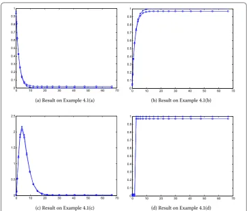
(a) Result on Example .(a) (b) Result on Example .(b)

[image:11.595.116.478.79.388.2]

(c) Result on Example .(c) (d) Result on Example .(d)

Figure 1 Numerical results on Example 4.1: ‘∗’ is the true solution and ‘◦’ denotes the approximate solution.

Example . The kernelKis given by

K(s,t) =e–st,

and the integration interval is [,∞). The true solutionf and the right-hand sideg are given by

(a) f(t) =e–t_, _g₍_s_{) =}  s+ .,

(b) f(t) =  –e–t_, _g₍_s_{) =}  s–

 s+ .,

(c) f(t) =t×e–t_, _g₍_s_{) =} 

(s+ .),

(d) f(t) =

, t≤,

, t> , g(s) = e–s

s .

The numerical results are displayed in Figure .

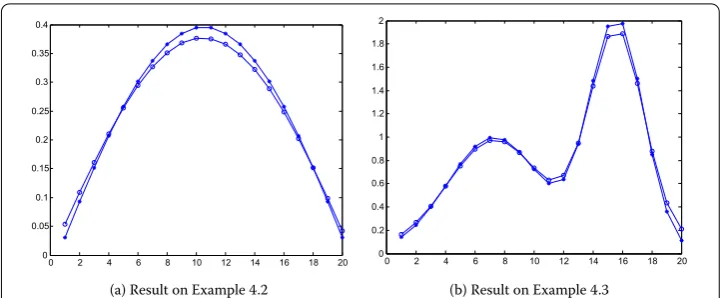
Example . Shaw test problem: one-dimensional image restoration model. We have the kernelKand the solutionf, which are given by

(12)

[image:12.595.117.478.81.230.2]

(a) Result on Example . (b) Result on Example .

Figure 2 Numerical results on Examples 4.2 and 4.3: ‘∗’ is the true solution and ‘◦’ denotes the approximate solution.

and

f(t) =a×exp

–c×(t–t)

+a×exp

–c×(t–t)

,

whereu=π×(sin(s) +sin(t)). BothKandf are discretized by simple quadrature to pro-duceAandx. Then the discrete right-hand side is produced asb=Ax. In our test, the constants are assigned as follows:a= ,c= ,t= .;a= ,c= ,t= –.. The nu-merical result is displayed in Figure (a).

Example . Baart test problem: the kernelKand right-hand sidegof the discretization of a ﬁrst-kind Fredholm integral equation are given by

K(s,t) =exps×cos(t), g(s) = ×sinh(s) s ,

wheres∈[,π/],t∈[,π]. The solution is given byf(t) =sin(t). The numerical result is displayed in Figure (b).

We can draw the conclusion from the above computational results: the proposed hybrid splitting method is valid and eﬃcient for the smoothing Tikhonov regularization problem.

5 Conclusions

(13)

updated. The proposed method is essentially to a hybrid splitting method since it com-bines the parallel splitting method and the alternating direction method, which are two power tools for the convex optimization problem with a separable structure. Under suit-able assumptions, the global convergence of the hybrid splitting method is proved. The numerical results on the discrete ill-posed problems show that the proposed method has validity and eﬃciency.

Competing interests

The authors declare that they have no competing interests.

Authors’ contributions

All authors contributed equally and signiﬁcantly in this paper. All authors read and approved the ﬁnal manuscript.

Author details

1_{College of Mathematics and Econometrics, Hunan University, Changsha, 410082, China.}2_{College of Mathematics and}

Computational Science, Hunan First Normal University, Changsha, 410205, China.3_{College of Mathematics and}

Computer Science, Fuzhou University, Fuzhou, 350108, China.

Acknowledgements

This work is supported by Natural Science Foundation of China (11571074), Natural Science Foundation of Fujian Province (2015J01010), Science and Technology Project of Hunan Province (2014SK3235), and Scientiﬁc Research Fund of Hunan Provincial Education Department (2015277).

Received: 3 December 2015 Accepted: 19 January 2016

References

1. Stephen, B, Lieven, V: Convex Optimization. Cambridge University Press, London (2004)

2. Achtziger, W, Hoheisel, T, Kanzow, C: A smoothing-regularization approach to mathematical programs with vanishing constraints. Comput. Optim. Appl.55(3), 733-767 (2013)

3. Lusem, AN, Svaiter, BF: A new smoothing-regularization approach for a maximum-likelihood estimation problem. Appl. Math. Optim.29(3), 225-241 (1994)

4. Chen, SF, Goodman, J: An empirical study of smoothing techniques for language modeling. Comput. Speech Lang.

13(4), 359-394 (1999)

5. Huber, PJ: Robust Statistics. Wiley-Interscience, New York (1981)

6. Tibshirani, R: Regression shrinkage and selection via the lasso. J. R. Stat. Soc., Ser. B58(1), 267-288 (1996) 7. Donoho, D: Compressed sensing. IEEE Trans. Inf. Theory52(4), 1289-1306 (2006)

8. Candes, EJ, Tao, T: Near optimal signal recovery from random projections: universal encoding strategies. IEEE Trans. Inf. Theory52(12), 5406-5425 (2006)

9. Zhang, Y: Theory of compressive sensing via1-minimization: a non-RIP analysis and extensions. J. Oper. Res. Soc.

China1(1), 79-105 (2013)

10. Chen, CH, He, BS, Ye, YY, Yuan, XM: The direct extension of ADMM for multi-block convex minimization problems is not necessarily convergent. Math. Program. (2014). doi:10.1007/s10107-014-0826-5

11. He, BS: Parallel splitting augmented Lagrangian methods for monotone structured variational inequalities. Comput. Optim. Appl.42(2), 195-212 (2009)

12. Peng, Z, Wu, DH: A partial parallel splitting augmented Lagrangian method for solving constrained matrix optimization problems. Comput. Math. Appl.60(6), 1515-1524 (2010)

13. Glowinski, R, Le Tallec, P: Augmented Lagrangian and Operator-Splitting Methods in Nonlinear Mechanics. SIAM Studies in Applied Mathematics. SIAM, Philadelphia (1989)

14. He, BS, Liao, LZ, Qian, MJ: Alternating projection based prediction-correction methods for structured variational inequalities. J. Comput. Math.24(6), 693-710 (2006)

15. He, BS, Xu, MH: A general framework of contraction methods for monotone variational inequalities. Pac. J. Optim.

4(2), 195-212 (2008)

16. Dai, YH, Fletcher, R: Projected Barzilai-Borwein methods for large-scale box-constrained quadratic programming. Numer. Math.100(1), 21-47 (2005)

17. Amir, B, Teboulle, M: A fast iterative shrinkage-thresholding algorithm for linear inverse problems. SIAM J. Imaging Sci.

2(1), 183-202 (2009)