R E S E A R C H
Open Access
An extended inequality approach for
evaluating decision making units
with a single output
Xiao-Li Meng
1,2and Fu-Gui Shi
1,2**Correspondence:
[email protected] 1School of Mathematics and
Statistics, Beijing Institute of Technology, Beijing, 100081, China 2Beijing Key Laboratory on MCAACI,
Beijing Institute of Technology, Beijing, 100081, China
Abstract
In this work, an extended evaluation approach for decision making units (DMUs) with a single output is proposed. Firstly, the input and output data for each DMU are changed in the same proportion until all the outputs are equal, and then the coordinate system is established with inputias theith coordinate axis. Secondly, in the coordinate system, the production possibility set, which is spanned by all the DMUs without the evaluated DMU, is expressed by inequalities. Moreover, the mathematical expression of the line segment joining the origin to the evaluated DMU is given. Thirdly, the efficiency measure of the evaluated DMU is obtained from the relationship between the production possibility set and the line segment. In order to distinguish the weak efficiency and efficiency, the partially ordered set and minimal element are introduced in the paper. Finally, an example is provided to illustrate the proposed approach.
Keywords: data envelopment analysis; decision making unit; inequality; partially ordered set; minimal element
1 Introduction
In recent years a great variety of scholarly efforts have been directed at the development of efficiency measures. These measures illustrate whether the decision making units (DMUs) are near the production frontier. Farrell [] seemed to be the first author who devoted his work to the study of the production frontier for evaluating productivity. A few years later, Farrell’s approach was developed to two major branches, including parametric es-timation method and non-parametric eses-timation method. Moreover, data envelopment analysis (DEA), which is used to estimate the efficiency of the evaluated DMU relative to peer DMUs, is the basic non-parametric estimation method. Since then, many improved approaches on DEA have been proposed [–].
What we focus on in this paper is the DEA with a single output. The initial DEA model (CCR model), as originally presented in [], was built on the earlier work of Farrell. This model allowed every DMU to select the most favorable weight while requiring the re-sulted ratios of weighted outputs to weighted inputs of all the DMUs to be not greater than . The CCR model is a fractional programming model and solved by transforming to a linear programming model. If the constraintnj=λj= is adjoined to the dual CCR
model, the extended model is known as BCC model []. Soon afterwards, Charneset al.
[] presented the CGSmodel to establish foundations of DEA for Pareto-Koopmans ef-ficient empirical production functions. Färe and Grosskopf introduced a non-parametric dual method (namely, FG model) to calculate the scale efficiency []. In , Seiford and Thrall [], who proposed the ST model, discussed the mathematical programming approach to frontier estimation, and examined the effect of model orientation on the ef-ficient frontier and the effect of convexity requirements on returns to scale. In addition, the transformations between models were provided.
Unlike the previous models, we develop an extended evaluation approach to estimate the efficiencies of DMUs with a single output. Different from DEA models, the proposed approach will estimate the efficiencies of DMUs only with changed input data rather than with the original input and output data. Moreover, efficiency of the evaluated DMU is estimated by considering the relationship between the defined production possibility set and the corresponding line segment of the evaluated DMU. Furthermore, the minimal element is introduced in the paper to distinguish the weak efficiency and efficiency.
The rest of the paper is unfolded as follows. The initial DEA model, partially ordered set and minimal element are reviewed in Section . In Section , the extended evaluation approach for DMUs with a single output is proposed. In Section , an example is given to illustrate the presented approach. In Section , results and discussion are given. The paper is concluded in Section .
2 An introduction to DEA model and the partially ordered set
As an extremely common DEA model, the CCR model assumes that there arenDMUs, and each DMU consumes the same type of inputs and produces the same type of outputs. Letm,rbe the numbers of inputs and outputs, respectively. All inputs and outputs are assumed to be nonnegative, and at least one input and one output are positive. The multi-ple inputs and outputs of each DMU are aggregated into a single virtual input and a single virtual output. The efficiency of the evaluated DMU is obtained as a ratio of its virtual output to its virtual input, and is subject to the condition that the ratio for each DMU is not greater than . The corresponding model is as follows:
(CCR) ⎧ ⎪ ⎪ ⎪ ⎪ ⎪ ⎪ ⎪ ⎪ ⎪ ⎨ ⎪ ⎪ ⎪ ⎪ ⎪ ⎪ ⎪ ⎪ ⎪ ⎩
maxuTy
vTx
s.t.
uTyj
vTxj ≤, j= , . . . ,j, . . . ,n,
u≥, u= ,
v≥, v= ,
()
linear model is obtained:
(PCCR) ⎧ ⎪ ⎪ ⎪ ⎪ ⎪ ⎪ ⎪ ⎪ ⎪ ⎪ ⎪ ⎨ ⎪ ⎪ ⎪ ⎪ ⎪ ⎪ ⎪ ⎪ ⎪ ⎪ ⎪ ⎩
maxμTy
s.t.
ωTxj–μTyj≥, j= , . . . ,n,
ωTx
= ,
ω≥, ω= ,
μ≥, μ= .
()
The essence of the model above is to find the weight vector to maximize its weighted output of the evaluated DMU, and the weighted output is not greater than the weighted input for every DMU. Moreover, the optimal objective values of DEA models vary in (, ]. The relationship between DEA efficiency and optimal objective value can be obtained as follows.
Definition If the optimal objective value of the evaluated DMU is equal to and there is at least one optimal solution in which the optimal weight vectors of inputs and outputs are greater than , then the evaluated DMU is DEA efficient.
Definition If the optimal objective value of the evaluated DMU is equal to and there is not any optimal solution in which the optimal weight vectors of inputs and outputs are greater than , then the evaluated DMU is weak DEA efficient.
Definition If the optimal objective value of the evaluated DMU is less than , then the evaluated DMU is DEA inefficient.
Subsequently, the partially ordered set and minimal element will be introduced. LetP
be a nonempty set. Any subset of the cartesian product setP×P={(x,y)|x,y∈P}is called a binary relation, denoted byR.a,b∈P,aRbif and only if (a,b)∈R[].
Definition A relation R is called a partial order on P if it satisfies, for allx,y,z∈P, () reflexivity,xRx,
() antisymmetry,xRyandyRximplyx=y, () transitivity,xRyandyRzimplyxRz.
A nonempty setPequipped with a partial order is called a partially ordered set, or poset for short. A partial orderRis traditionally replaced by ‘≤’. That is, we usually replacexRy
byx≤ywhich is read as ‘xis less than or equal toy’.
Definition Suppose thatPis a partially ordered set andQ⊆P,a∈Qis called a minimal element ofQifa≥xandx∈Qimplya=x.
For any nonempty finite subsetS⊆P, there exists at least one minimal elementx∈S.
3 The extended evaluation approach
It should be noted that all DMUs used from this section onwards are in the form of a single output. Now suppose there arenDMUs withminputs and one output. Especially,
Xk={xk, . . . ,xkm}denotes the input vector of thekth DMU withkranging from ton.
Without loss of generality,Yk={yk}is the output vector with a single element for thekth
DMU. Since efficiency is independent of the changes of inputs and output by the same proportion, then we change the input and output data of each DMU in the same propor-tion until the output data of all DMUs are equal. The input vector and output vector of the
kth DMU are transformed intoXk={¯xk, . . . ,x¯km}andYk={¯yk}=Yl,l= , . . . ,n. In order
to discuss the convenience of the problem, the output state will not be considered in the evaluation approach.
Next, we define the production possibility set Ti which is spanned by all the DMUs without theith evaluated DMU. For instance, if there are five DMUs (i.e., DMU, DMU, DMU, DMU, and DMU), and DMUis the evaluated DMU, then the production pos-sibility setTis spanned by DMU, DMU, DMU, and DMU. Moreover, the production possibility setTisatisfies the following conditions:
() Xk∈Ti,k=i.
() For arbitraryXk,Xl∈Ti, andα∈[, ], we haveαXk+ ( –α)Xl∈Ti. () IfXk∈Ti, andXl≥Xk, thenXl∈Ti.
() IfXk∈Ti, andα≥, thenαXk∈Ti.
() Tiis the least set which satisfies the conditions ()–().
The production possibility setTi spanned byXk={¯xk, . . . ,xkm¯ }, k=iis given by the following formula:
Ti=
X n
k=,k=i
λkXk≤X,λk≥, n
k=,k=i λk=
, i= , . . . ,n. ()
3.1 The relationship between the defined production possibility set and the line segment for the evaluated DMU
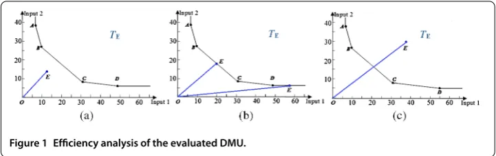
To better show the proposed approach, we will consider the case with two inputs and one output. Then we change the inputs and output of each DMU in the same proportion until output data of all the DMUs are equal. Next, the coordinate system is established with input and input as thexandycoordinate axes. For the DMU under evaluation, the closer it gets to the coordinate origin, the higher production efficiency will be.
In this section, there are five DMUs (i.e., DMUsA,B,C,DandE) with the same output data, and DMUE is the evaluated DMU, then the production possibility set is spanned by DMUsA,B,CandD. As shown in Figure , the solid line segments connecting points
A,B,CandDconstitute an isoquant that represents the different input amounts to pro-duce the same output amount. Since it is impossible to repro-duce the amount of one of the inputs without increasing another input amount if one is to stay on this isoquant, the solid line segments represent the efficient production frontier [] of the production possibility setTE.
From Figure (a) we can see that the evaluated DMUEis closer to the coordinate ori-gin than the production frontier (that is to say, the line segmentOEand the production possibility setTEare disjoint). There exist the optimal weight vectors of inputs and output
Figure 1 Efficiency analysis of the evaluated DMU.
efficient if there is no solution of the inequalities of the production possibility setTEand
the line segmentOE.
In Figure (b), the evaluated DMUEis located on the production frontier (namely, the line segmentOEmeets on the production possibility setTEat a pointE, and there is exactly one solution of the inequalities of the production possibility setTEand the line segment
OE). There are two cases of interest: () The evaluated DMUsE on the three solid line segmentsAB,BCandCDare efficient. () The evaluated DMUsEon the two rays issuing from the pointsAandDare weakly efficient [, ]. It is important to stress here that at least one input of the weakly efficient DMU is strictly greater than that of an efficient DMU. Moreover, if the order relation≤for DMUsA,B,C,DandEis reflective, antisymmetric and transitive in the coordinate system, then the set{A,B,C,D,E}is a partially ordered set. In the proposed approach, with the same output for all DMUs, if an evaluated DMU is located on the production frontier, its efficiency is dependent on whether the evaluated DMU is a minimal element or not. An evaluated DMU on the production frontier is weakly efficient if it is not a minimal element, otherwise the evaluated DMU is efficient.
Refer to Figures (c), since DMUEis farther from the coordinate origin than the pro-duction frontier, that is, the line segmentOEmeets on the production possibility setTE
at more than one point, DMUEis located in the defined production possibility setTE, thus DMUEis inefficient. In such a case, the solution of inequalities of the production possibility set and the line segment is not unique.
From the analysis mentioned above, the conclusion thus noted may be recorded as
Theorem Suppose there are n DMUs(i.e.,DMU E, . . . ,En)with m inputs and one
out-put,and output data of all DMUs are equal.Then an m-dimensional coordinate system is established with input i as the ith coordinate axis,the point Ekstands for the kth DMU in the coordinate system,and OEkdenotes the line segment from the origin to Ek.Tk,spanned by other n– DMUs,is the production possibility set of the kth DMU.Efficiency is obtained from the relationship between line segment OEkand the production possibility set Tkfor the kth evaluated DMU is as follows:
() If the line segmentOEkand the production possibility setTkare disjoint,that is,there is no solution of the inequalities of the production possibility setTkand the line segmentOEk,then thekth DMU is efficient.
() The line segmentOEkmeets on the production possibility setTkat the pointEk,
() If the line segmentOEkmeets on the production possibility setTk,and the number of points of intersection are greater than one,that is,the number of solutions of the inequalities of the production possibility setTkand the line segmentOEkis greater than one,then thekth DMU is inefficient,andEkis located in the production possibility set.
Notice that the number of points of intersection ofOEkandTkis equal to the number of
solutions of equation () and the expressions of line segmentOEk. If the input vector of DMUEkisXk={¯xk, . . . ,xkm¯ }, the expressions of line segmentOEkare as follows:
⎧ ⎪ ⎪ ⎪ ⎪ ⎪ ⎪ ⎪ ⎪ ⎪ ⎨ ⎪ ⎪ ⎪ ⎪ ⎪ ⎪ ⎪ ⎪ ⎪ ⎩
¯ x=λx¯k,
¯
x=λxk¯ , ..
.
¯
xm=λxkm¯ ,
λ∈(, ].
4 Numerical experiments
In this section, an example is given to illustrate the practical relevance of the presented approach. In the example, there are five DMUs (i.e., DMUsA,B,C,DandE) with two inputs and a single output listed in Table .
At first, we change the inputs and output of every DMU in the same proportion until the output data are equal to , and establish the coordinate system with input and input as thexandycoordinate axes. The dots (•) denote the corresponding DMUs with the same output.
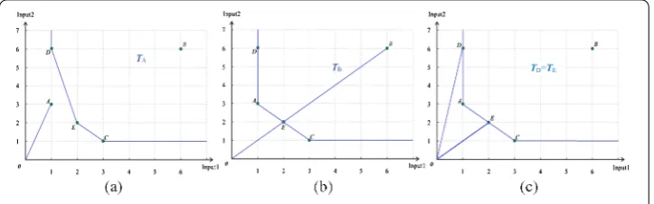
Next, the DMUAwill be estimated, and the evaluation process is as follows. The pro-duction possibility setTAis spanned by DMUsB,C,DandE(see Figure (a)). By using
equation (), we get the following expression:
TA=
X
k=
λkXk≤X,
k=
λk= ,λk≥,k= , , ,
,
that is,
⎧ ⎪ ⎪ ⎪ ⎪ ⎪ ⎨ ⎪ ⎪ ⎪ ⎪ ⎪ ⎩
λ+ λ+λ+ λ≤ ¯x,
λ+λ+ λ+ λ≤ ¯x,
λ+λ+λ+λ= ,
λk≥, k= , , , .
()
Table 1 DMUs with two inputs and a single output
DMU A B C D E
Input 1 2 3 9 1 4
Input 2 6 3 3 6 4
Figure 2 Efficiency analysis of DMUsA,B,DandE.
In addition, the expressions of line segmentOAare
⎧ ⎪ ⎪ ⎨ ⎪ ⎪ ⎩ ¯ x=λ,
¯ x= λ,
λ∈(, ].
()
The relationship between the line segmentsOAand the production possibility setTAfor
the evaluated DMUAwill be analyzed. As shown in Figure (a), the line segmentsOAand the production possibility setTAare disjoint, and there is no solution for inequalities () and (). By applying Theorem , we conclude that DMUAis efficient.
⎧ ⎪ ⎪ ⎪ ⎪ ⎪ ⎪ ⎪ ⎪ ⎪ ⎪ ⎪ ⎪ ⎪ ⎪ ⎨ ⎪ ⎪ ⎪ ⎪ ⎪ ⎪ ⎪ ⎪ ⎪ ⎪ ⎪ ⎪ ⎪ ⎪ ⎩
λ+ λ+λ+ λ≤ ¯x,
λ+λ+ λ+ λ≤ ¯x,
λ+λ+λ+λ= ,
λk≥, k= , , , ,
λ=x¯,
λ=x¯,
λ∈(, ].
()
Similarly, the production possibility set TB of the evaluated DMUBis shown in Fig-ure (b), and the inequalities of the production possibility setTBand line segmentOBare
expressed by (). In Figure (b), we see that DMUBis located in the production possibility setTB, while there are infinite solutions for (), so DMUBis inefficient.
⎧ ⎪ ⎪ ⎪ ⎪ ⎪ ⎪ ⎪ ⎪ ⎪ ⎪ ⎪ ⎪ ⎪ ⎪ ⎨ ⎪ ⎪ ⎪ ⎪ ⎪ ⎪ ⎪ ⎪ ⎪ ⎪ ⎪ ⎪ ⎪ ⎪ ⎩
λ+ λ+ λ+ λ≤ ¯x,
λ+ λ+λ+ λ≤ ¯x,
λ+λ+λ+λ= ,
λk≥, k= , , , ,
λ=x¯,
λ=x¯,
λ∈(, ].
Table 2 The efficiencies of DMUs
DMU A B C D E
DEA efficiency of model (2) DEA efficient DEA inefficient DEA efficient Weak DEA efficient DEA efficient Efficiency of the proposed
approach
Efficient Inefficient Efficient Weak efficient Efficient
The same spanning production possibility sets of DMUsDandEare shown in Figure (c), the inequalities of DMUsDandE are expressed by () and () separately. The two line segmentsODandOEmeet on the production possibility setTD=TEat the production frontier, and there is only one solution for () and (), respectively. In addition, the data of Input of DMUsDandAare equal, but the data of Input of DMU Dare greater than those of DMUA, and DMUDis not a minimal element of{A,B,C,D,E} with the order relation≤, so DMUDis weakly efficient. DMUEis a minimal element of partially ordered set{A,B,C,D,E}, so it is efficient. Moreover, DMUEcan be expressed by a linear combination of DMUAandC.
⎧ ⎪ ⎪ ⎪ ⎪ ⎪ ⎪ ⎪ ⎪ ⎪ ⎪ ⎪ ⎪ ⎪ ⎪ ⎨ ⎪ ⎪ ⎪ ⎪ ⎪ ⎪ ⎪ ⎪ ⎪ ⎪ ⎪ ⎪ ⎪ ⎪ ⎩
λ+ λ+ λ+λ≤ ¯x,
λ+ λ+λ+ λ≤ ¯x,
λ+λ+λ+λ= ,
λk≥, k= , , , ,
λ=x¯,
λ=x¯,
λ∈(, ].
()
At last, by a similar evaluation process, we consider the DMUC, and the result is shown in Table . We can see that the evaluation results are consistent with the results from model ().
5 Results and discussion
6 Conclusions
The results of the proposed approach are consistent with the results of the DEA model. It is worthy of note that the inequality approach can also be applied to super-efficiency DEA. If there is no solution for the inequalities, the evaluated DMU is super-efficient. If the solution of inequalities is not unique, the evaluated DMU is inefficient. If there is exactly one solution, and the evaluated DMU is a minimal element of all the DMUs, then the evaluated DMU is efficient, otherwise the evaluated DMU is weakly efficient.
Acknowledgements
This research was supported by the National Natural Science Foundation of China (11371002) and Specialized Research Fund for the Doctoral Program of Higher Education (20131101110048).
Competing interests
The authors declare that there are no competing interests.
Authors’ contributions
All authors contributed equally and significantly in writing this paper. All authors read and approved the final manuscript.
Publisher’s Note
Springer Nature remains neutral with regard to jurisdictional claims in published maps and institutional affiliations.
Received: 16 May 2017 Accepted: 21 July 2017
References
1. Farrell, MJ: The measurement of productive efficiency. J. R. Stat. Soc. A120, 253-281 (1957)
2. Banker, RD, Morey, RC: Efficiency analysis for exogenously fixed inputs and outputs. Oper. Res.34, 513-520 (1986) 3. Charnes, A, Cooper, WW, Wei, QL, Huang, ZM: Cone ratio data envelopment analysis and multi-objective
programming. Int. J. Syst. Sci.20, 1099-1118 (1989)
4. Wei, QL, Yan, H: Congestion and return to scale in data envelopment analysis. Eur. J. Oper. Res.153, 641-660 (2004) 5. Meng, XL, Shi, FG: An extended DEA with more general fuzzy data based upon the centroid formula. J. Intell. Fuzzy
Syst.33, 457-465 (2017)
6. Andersen, P, Petersen, NC: A procedure for ranking efficient units in data envelopment analysis. Manag. Sci.39, 1261-1264 (1993)
7. Lins, MPE, Gomes, EG, Soares de Mello, JCCB, Soares de Mello, AJR: Olympic ranking based on a zero sum gains DEA model. Eur. J. Oper. Res.148, 312-322 (2003)
8. Yang, F, Wu, DD, Liang, L, Liam, O: Competition strategy and efficiency evaluation for decision making units with fixed-sum outputs. Eur. J. Oper. Res.212, 560-569 (2011)
9. Saraçli, S, Kiliç, ˙I, Do ˇgan, ˙I, Gazelo ˇglu, C: An application of data envelopment analysis on marble factories. J. Inequal. Appl.2013, Article ID 139 (2013)
10. Yang, M, Li, YJ, Chen, Y, Liang, L: An equilibrium efficiency frontier data envelopment analysis approach for evaluating decision-making units with fixed-sum outputs. Eur. J. Oper. Res.239, 479-489 (2014)
11. Banker, RD, Chang, H, Zheng, Z: On the use of super-efficiency procedures for ranking efficient units and identifying outliers. Ann. Oper. Res.250, 21-35 (2017)
12. Yang, M, Li, YJ, Liang, L: A generalized equilibrium efficient frontier data envelopment analysis approach for evaluating DMUs with fixed-sum outputs. Eur. J. Oper. Res.246, 209-217 (2015)
13. Zanella, A, Camanho, AS, Dias, TG: Undesirable outputs and weighting schemes in composite indicators based on data envelopment analysis. Eur. J. Oper. Res.245, 517-530 (2015)
14. Aleskerov, F, Petrushchenko, V: DEA by sequential exclusion of alternatives in heterogeneous samples. Int. J. Inf. Technol. Decis. Mak.15, 5-22 (2016)
15. Kao, C: Measurement and decomposition of the Malmquist productivity index for parallel production systems. Omega67, 54-59 (2017)
16. Mardani, A, Zavadskas, EK, Streimikiene, D, Jusoh, A, Khoshnoudi, M: A comprehensive review of data envelopment analysis (DEA) approach in energy efficiency. Renew. Sustain. Energy Rev.70, 1298-1322 (2017)
17. Charnes, A, Cooper, WW, Rhodes, E: Measuring the efficiency of decision making units. Eur. J. Oper. Res.2, 429-444 (1978)
18. Banker, RD, Charnes, A, Cooper, WW: Some models for estimating technical and scale inefficiencies in data envelopment analysis. Manag. Sci.30, 1078-1092 (1984)
19. Charnes, A, Cooper, WW, Golany, B, Seiford, L, Stutz, J: Foundations of data envelopment analysis for Pareto-Koopmans efficient empirical production functions. J. Econom.30, 91-107 (1985)
20. Färe, R, Grosskopf, S: A nonparametric cost approach to scale efficiency. Scand. J. Econ.87, 594-604 (1985) 21. Seiford, LM, Thrall, RM: Recent development in DEA: the mathematical programming approach to frontier analysis.
J. Econom.46, 7-38 (1990)
22. Charnes, A, Cooper, WW: Programming with linear fractional functionals. Nav. Res. Logist.9, 181-186 (1962) 23. Davey, BA, Priestley, HA: Introduction to Lattices and Order, pp. 1-18. Cambridge University Press, Cambridge (2002) 24. Yu, G, Wei, QL, Brockett, P, Zhou, L: Construction of all DEA efficient surfaces of the production possibility set under
25. Wei, QL, Yan, H: Characteristics and structures of weak efficient surfaces of production possibility sets. J. Math. Anal. Appl.327, 1055-1074 (2007)