R E S E A R C H
Open Access
Superconvergence of the local
discontinuous Galerkin method for nonlinear
convection-diffusion problems
Hui Bi
*and Chengeng Qian
*Correspondence: [email protected] Department of Applied Mathematics, Harbin University of Science and Technology, Harbin, 150080, China
Abstract
In this paper, we discuss the superconvergence of the local discontinuous Galerkin methods for nonlinear convection-diffusion equations. We prove that the numerical solution is (k+ 3/2)th-order superconvergent to a particular projection of the exact solution, when the upwind flux and the alternating fluxes are used. The proof is valid for arbitrary nonuniform regular meshes and for piecewise polynomials of degreek
(k≥1). The numerical experiments reveal that the property of superconvergence actually holds true for general fluxes.
Keywords: local discontinuous Galerkin method; superconvergence; convection-diffusion equations
1 Introduction
In this paper, we discuss the nonlinear convection-diffusion equations given by
ut+∂xf(u) =νuxx, (x,t)∈[, π]×[,T],
u(x, ) =u(x), x∈[, π],
(.)
with the periodic boundary condition, whereν> is a constant. We study the supercon-vergence of the local dicontinuous Galerkin (LDG) solutions towards a particular projec-tion of the exact soluprojec-tion.
The high-order numerical methods have been applied in a variety of fields [–]. The LDG method is one of those numerical methods, which were first constructed by Cock-burn and Shu and motivated by Bassi and Rebay [, ] to solve the convection-diffusion equations. Since then, the LDG method has been used to solve the time-dependent equa-tions with high spatial derivatives, such as the Korteweg-de Vries (KdV) equaequa-tions [], time-dependent fourth-order problems [] and the general fifth-order KdV equations []. See more details in []. We now state some theoretical results, which represent the cru-cial technique to treat the nonlinear parts of the equations. In [], Zhang and Shu study the error estimate of the discontinuous Galerkin (DG) method with second-order Runge-Kutta time discretization. They obtain the optimal error estimate of the (k+ )th order for upwind numerical fluxes and a suboptimal error estimate of the (k+ /)th order for gen-eral monotone fluxes, wherekis the order of the piecewise polynomial space. The proof
holds true for arbitrary meshes under the reasonable assumptions. Then Zhang and Shu extend the results in [] to the third-order TVD Runge-Kutta time discretization case, which is more popular in the computation []. In [], Wang and Shu obtain the opti-mal error estimate of the LDG method with implicit-explicit time-marching for nonlinear convection-diffusion problems, when the fluxes are chosen to be the general monotone fluxes and alternating fluxes. In the above three papers, the Taylor expansion and ana prioriassumption are used to estimate the nonlinear parts.
We would like to mention the superconvergence results for DG and LDG methods. In [], Cheng and Shu study the superconvergence of the (k+ /)th order of the DG solu-tion towards a particular projecsolu-tion for linear conservasolu-tion laws. The limitasolu-tions of [] are that the proof is only valid for uniform meshes and linear piecewise polynomial space. Cheng and Shu overcome this limitation in [], which implies that the result in [] holds true for arbitrary meshes andkth-order finite element spaces. Cheng and Shu also extend the result to the linear convection-diffusion problems. For the linear equations with high-order spatial derivatives, Hufford obtains the superconvergence of the (k+ /)th order for linear KdV equations [] and Meng gets the same result for the linear fourth-order problems []. But for above linear problems, the numerical experiments imply that the numerical solution is superconvergent to the exact solution at a rate of the (k+ )th order. It is highly nontrivial to obtain this half-order increase theoretically. For linear conserva-tion laws and linear parabolic equaconserva-tions, Yang and Shu use a new technique to carry out the optimal order of the superconvergence [, ]. In addition, they prove that DG and LDG solutions are (k+ )th-order superconvergent to the exact solutions at Radau points. In [–], Cao and Zhang present another framework to demonstrate the superconver-gence at Radau points for linear -D and -D hyperbolic problems and -D linear parabolic problems. The first superconvergence proof with the DG method for nonlinear conserva-tion laws is obtained in [], when the upwind fluxes are used, under the condiconserva-tion that the absolute value of the convection termf has a positive low bound. In this paper, we obtain a similar result for the nonlinear convection-diffusion problems, when the upwind fluxes and alternating fluxes are used under the assumption that|f| ≥. Due to the char-acter of the LDG method, there is no need of a strict positive bound of the absolute value of the convection term. In [], Cao obtains the superconvergence of DG methods based on upwind-biased fluxes for -D linear hyperbolic equations. Guo and Yang show the DG solution is (k+ )th-order accurate at the downwind points and (k+ )th-order accurate at all the other downwind-biased Radau points in [].
The outline of this paper is as follows. In Section , we present the semi-discrete LDG schemes for nonlinear convection-diffusion problems. In Section , we state the main proofs of our theorems. Some numerical experiments are presented in Section , and in Section , we give the conclusion and our future work. Finally, we give a proof of a lemma in the Appendix.
2 The local discontinuous Galerkin method for nonlinear convection-diffusion equations
2.1 The local discontinuous Galerkin method
In this subsection, we will present the semi-discrete LDG method for equation (.). We first divide the computational domain= [, π] intoNsubintervals. We have
We denote each subinterval byIj= [xj–/,xj+/] and the union of allIjbyIh. Lethj=xj+/–
xj–/be the length of the subinterval andh=max≤j≤Nhj. We denote the left and right limits of the functionvhat the element interfacexj+/by (vh)–j+/and (vh)+j+/, respectively.
We also set [vh]j+/= (vh)+j+/– (vh)–j+/and denote the center ofIjbyxj= (xj+/+xj–/)/.
We would like to assume our mesh is regular, which means that there exists a constant λ> such thatλh<hj.
We choose the finite element space as thekth-order piecewise polynomial space that is denoted by
Vhk=vh:vh|Ij∈P
k(I j)
,
wherePk(I
j) is the space of polynomials of degree at mostkonIj. In addition, we define the broken Sobolev space on= [, π] as
Hl h=
φ:φ|Ij∈H
l,(I
j)
.
Before we construct the LDG method, we need an auxiliary variableq, so we rewrite equation (.) as a first-order system. We have
ut+∂xf(u) = √
νqx, (.a)
q=√νux. (.b)
Then the semi-discrete LDG scheme is formulated as follows: finduh,qh∈Vhksuch that for anywh,vh∈Vhk
Ij
(uh)tvhdx+fˆ
u–h,u+hv–hj+/–fˆu–h,uh+v+hj–/–
Ij
f(uh)(vh)xdx
=√ν
ˆ
qhv–hj+/–qˆhv +
hj–/–
Ij
qh(vh)xdx , (.a)
Ij
qhwhdx= √
ν
ˆ
uhw–hj+/–uˆhw +
hj–/–
Ij
uh(wh)xdx , (.b)
wherefˆ(a,b) is usually a monotone flux, which satisfies:
• fˆ(a,b)is consistent with the physical fluxf, namelyfˆ(p,p) =f(p). • fˆ(a,b)is a Lipschitz continuous function in both arguments.
• fˆ(a,b)is a nondecreasing function inaand a nonincreasing function inb. Hereuˆh,qˆhare the alternating fluxes, of which we have two choices:
ˆ
uh=u–, qˆh=q+, (.)
ˆ
uh=u+, qˆh=q–. (.)
that we could use the upwind flux. We have
ˆ
fp–h,p+h=
⎧ ⎨ ⎩
f(p–
h), f(ph)≥,
f(p+h), f(ph) < .
2.2 Norms
In this subsection, we give some norms used in this paper. We denote the standard L
norm onIjby · Ij. Then the norm of Sobolev spaceH
l(I
j) is defined as
ul,Ij=
≤α≤l
Dαu
Ij
/
,
wherelis a natural number and Dαis theαth-order spatial derivative operator.
We denote the norm ofHlhby
ul=
N
j=
ul,Ij
/
.
For convenience, we set · = · . Moreover, theL∞norm of the whole computational
domain is
u∞= max
≤j≤Nu∞,Ij,
whereu∞,Ij is the standardL∞ norm onIj. The norm on the boundary ofIjis defined
as
u∂Ij=
u–hj+/+u+hj–//.
Then we have
u∂Ih=
N
j=
u∂Ij
/
.
2.3 Properties of the finite element space
We first present the Gauss-Radau projections, fromHk+
h intoVhk, which are denoted by
P–
handP+h. Ifk≥, we define thePh–uto be the projection ofuintoVhk, such that for anyIj
Ij
u–P–huvhdx= , ∀vh∈Pk–(Ij), (.a)
P–hux–j+/=u–j+/. (.b)
In addition, we defineP+
huas
Ij
u–P+huvhdx= , ∀vh∈Pk–(Ij), (.a)
P+hux+j–/=u+j–/, (.b)
We denote the projection error (u–P–
hu) or (u–P+hu) byηu. Thanks to the standard approximation theory [], it is easy to obtain the following approximation property. Sup-poseu(x)∈Hk+(I
j) and is sufficiently smooth. Then we have
ηuIj+h
/η
u∞,Ij+h
/η
u∂Ij≤Ch
k+
j , (.)
whereCis a positive constant independent ofhj.
Here and below, we useCto denote the corresponding constant of the estimate for
projection errors. Now we turn to the three inverse properties of the finite element space
Vk
h. For anyvh∈Vhk, there exists a positive constantμindependent ofhandj, such that
(vh)xI
j≤μh
–v
hIj, (.a)
vh∂Ij≤μh
–/v
hIj, (.b)
vh∞,Ij≤μ
–/h–/v
hIj. (.c)
For more details on these inverse properties, we refer the reader to [].
2.4 Initial projection
In order to complete the proof, an initial condition compatible with the superconvergence order would be constructed with care. Fortunately, a (k+ /)th-order initial conditionPh presented in [] is valid in our proof, that is, for any functionu,Phu∈Vhk. Moreover, we supposeqh∈Vhkis the unique solution to
Ij
qhwhdx= (Phu)h–w–hj+/– (Phu) –
hw+hj–/–
Ij
Phuh(wh)xdx,
for anyIj. Also, we require
Ij
Ph–u–Phu
vhdx=
Ij
Ph+q–qh
vhdx, ∀vh∈Pk–(Ij), (.)
(u–Phu)–j+/= (q–qh)+j+/. (.)
We would like to remark thatPhexists and is unique. Moreover, we have the following estimate:
Ph–u–Phu≤CIPhk+/, (.)
whereCIP=CIP(uk+,λ) is a positive constant.
3 Superconvergence
In this section, we will give the main proof of superconvergence. Similar to [], we assume that the exact solutionu(x,t) is sufficiently smooth. We have
whereSis a constant independent oftandh. Also, the flux functionf is smooth enough, for examplef ∈C, and its derivatives are bounded onR. We have
f(p),f(p),f(p)≤Cm, ∀p∈R. (.)
We would like to remark that this assumption is reasonable with the original or a suitably modified fluxf, if we only consider the smooth solution. See for more details [].
Without loss of generality, we assumef> andν= . Then the fluxes are chosen as
ˆ
fu–h,uh+=fu–h, uˆh=u–h, qˆh=q+h. (.)
For ease of notation, we denote the error between the exact solutionuand the numerical solutionuhbyeu=u–uh. Also, we set
ξu=P–hu–uh=eu–ηu,
ξq=P+hq–qh=eq–ηq.
Next, we will introduce three operators, namely,
H–
j(w,v) =
Ij
wvxdx–w–v–j+/+w–v+j–/,
H+
j(w,v) =
Ij
wvxdx–w+v–j+/+w+v+j–/,
Kj(w,v) =
Ij
f(w)vxdx–f
w–v–j+/+fw–v+j–/.
When the fluxes (.) are used, we rewrite (.a)-(.b) as
Ij
(uh)tvhdx–Kj(uh,vh) = –H+j(qh,vh), (.a)
Ij
qhwhdx= –Hj–(uh,wh). (.b)
Foru,qare exact solutions, we get a similar system to (.a)-(.b), which is
Ij
utvhdx–Kj(u,vh) = –H+j(q,vh), (.a)
Ij
qwhdx= –H–j(u,wh). (.b)
Then we obtain the error equations
Ij
(eu)tvhdx=Kj(u,vh) –Kj(uh,vh) –Hj+(eq,vh), (.a)
Ij
Due to the properties of Gauss-Radau projections and summing (.a)-(.b) overj, we obtain
(eu)tvhdx=K(u,vh) –K(uh,vh) –H+(ξq,vh), (.a)
eqwhdx= –H–(ξu,wh), (.b)
whereK=Nj=KjandH±=Nj=H±j .
Now we turn to an investigation of the properties ofH±(·,·) andK(·,·). By integrating by parts, we get
H–
j(w,v) = –
Ij
wxvdx– [w]j–/v+j–/, (.)
H+
j(w,v) = –
Ij
wxvdx– [w]j+/v–j+/. (.)
Under the periodic conditions, we have the following equation:
H–(w,v) +H+(v,w) = , (.)
whose proof is straightforward.
For the nonlinear part, the derivation of the estimate is a little involving. We would like to remark that the following estimate inequality is not the final form, since we will adjust it further to obtain the suitable form in different proofs.
Lemma Under the assumptions(.)and(.), we have the following estimate of the nonlinear part.For any vh∈Vhk,
K(u,vh) –K(uh,vh)≤Cfhηu(vh)x+Cf
ξq+ξu+h–eu∞eu
vh
+ N
j=
f(uj–/)
Ij
ηqvhdx
, (.)
whereCf is a constant dependent on|f|,|f|,μand the exact solution u,but independent
of h.
Proof We begin with using the second-order Taylor expansion with respect to the vari-ableu. We have
f(u) –f(uh) =f(u)ηu+f(u)ξu– Rfe
u, (.)
f(u) –fu–h=f(u)ξu–+f(u)ηu–– R˜f
e–u, (.)
where
Rf =f
αu+ ( –α)uh α∈(, )
, ˜
Rf =f
˜
We remark that we have removed the subscript (j+ /) in (.) for notational conve-nience.
Noting that (η–u)j+/= , we divide (K(u,vh) –K(uh,vh)) into three parts. We have
K(u,vh) –K(uh,vh)≤ |++|
≤ ||+||+||,
where
=
N
j=
Ij
f(u)ηu(vh)xdx,
=
N
j=
Ij
f(u)ξu(vh)xdx–f(u)ξu–v–hj+/+f
(u)ξ–
uv+hj–/,
= –
N
j=
Ij
Rfeu(vh)xdx–R˜f
e–uv–hj+/+R˜f
e–uv+hj–/
.
We will estimate these three parts below: • The estimate of||.
Due to property (.a)-(.b), we have
=
N
j=
Ij
f(u) –f(uj)
ηu(vh)xdx.
For|f|is bounded, it is easy to show that|f(u) –f(uj)| ≤Cfh. Then we employ the Cauchy-Schwarz inequality to obtain
|| ≤Cfhηu(vh)x. (.)
• The estimate of||.
Proceeding as in the estimate of||, we split the integration into two parts. We
have
=
N
j=
Ij
f(u) –f(uj–/)
ξu(vh)xdx
–f(uj+/) –f(uj–/)
ξu–v–hj+/
+f(uj–/)
Ij
ξu(vh)xdx–ξu–v–hj+/+ξ –
uv+hj–/ .
Noting that
Ij
ξu(vh)xdx–ξu–v–hj+/+ξ –
uv+hj–/= –
with straightforward application of the Cauchy-Schwarz inequality and using properties (.a) and (.c), we obtain
|| ≤
N
j=
ChξuIj(vh)xIj+f
(u
j–/)ξqIjvhIj
+f(uj–/)
Ij
ηqvhdx
+Chξu∂Ijvh∂Ij
≤Cf
ξu+ξq
vh+ N
j=
f(uj–/)
Ij
ηqvhdx
. (.)
• The estimate of||.
Applying the Cauchy-Schwarz inequality, we obtain
|| ≤
N
j=
Ceu∞euIj(vh)xIj+Ceu∞eu∂Ijvh∂Ij
≤Ceu∞eu(vh)x+Ceu∞eu∂vh∂.
In accordance with properties (.b) and (.c), we have
|| ≤Cfh–eu∞euvh. (.)
Collecting (.), (.) and (.), we obtain the estimate (.).
We would like to remark that the estimate is also valid on each elementIj, though we only present the result on the whole computational domain. Now we move on to the error estimate of semi-discrete LDG schemes.
Lemma Suppose that u,q are the exact solutions of system(.a)-(.b),which are suffi-ciently smooth,and that uh,qhare the solutions of(.a)-(.b).Under assumptions(.)
and(.),we have the following estimate:
d dtξu
+ξ
q≤Cf(Cf+ +Ce)ξu+Chk+, (.)
whereCe=h–eu∞+h–eu∞andCis a constant independent of h.
Proof Taking (vh,wh) = (ξu,ξq) and adding up (.a) and (.b), we have
d dtξu
+ξ
q=K(u,ξu) –K(uh,ξu) –
(ηu)tξudx–
ηqξqdx
–H+(ξq,ξu) –H–(ξu,ξq). (.)
We deduce from property (.) that
which implies that
d dtξu
+ξ
q≤K(u,ξu) –K(uh,ξu)+
(ηu)tξudx
+
ηqξqdx
. (.)
On the other hand, plugging vh=ξu back into (.), applying the Cauchy-Schwarz in-equality to the integration term and using property (.a), we obtain
K(u,ξu) –K(uh,ξu) ≤μCfηuξu+Cf
ηqξu+ξqξu+ξu
+Cfh–eu∞euξu. (.)
Now we turn to the estimate of the last term on the right hand side of (.), as follows:
h–eu∞euξu ≤h–eu∞
ηu+ξu
ξu ≤h–eu∞ξu+Chkeu∞ξu
≤ C
hk++Ceξu, (.)
whereCe=h–eu∞+h–eu∞. In the first step, we use the triangle inequality and prop-erty (.). The proof of the last step is an application of Young’s inequality. Then we employ property (.) and Young’s inequality to get
K(u,ξu) –K(uh,ξu)≤CKhk++ξq+Cf(Cf+ +Ce)ξu, (.)
where CK= μC
fC+CfC. Finally, applying property (.), the Cauchy-Schwarz
in-equality and Young’s inin-equality, we have
(ηu)tξudx
+
ηqξqdx
≤Chk+
ξu+ξq
≤ ˜Chk++Cfξu+ ξq
. (.)
Collecting (.) and (.), we arrive at (.). We thus finish our demonstration.
To estimateeuandeq, we would like to follow [] to make thea prioriassumption that, ifhis sufficiently small, we have
ξu ≤h. (.)
It follows from property (.c), property (.) and the triangle inequality that
eu ≤(C+ )h, ξu∞≤μ/h/, eu∞≤
C+μ–/
h/. (.)
If assumption (.) is true, then there exists a positive constantδsuch that
Ce=h–eu∞+h–eu∞≤δ, (.)
which implies that
d dtξu
+ξ
q≤ ˆCξu+Chk+, (.)
whereCˆ=Cf(Cf+ +δ).
By using the Gronwall inequality and the triangle inequality, we obtain the error estimate as follows:
ξu ≤Chk+, eu ≤Chk+, eq ≤Chk+, (.)
whereCis a constant associated with|f|,|f|,μ, the exact solutionuand the final timeT. In addition, we give a lemma to estimate(eu)t, which will be proved in the Appendix.
Lemma Under the assumptions(.), (.)and(.),we have the following estimate:
(eu)t≤Chk+. (.)
Next we will present a crucial lemma which will be used to derive the superconvergence.
Lemma Suppose assumptions(.), (.)and(.)are true.Then we have the following inequalities:
(ξu)xIj≤CseqIj, (.)
(ξq)xIj≤Cs
ηuIj+ηqIj+(eu)tIj+ξqIj+ξuIj+euIj
, (.)
whereCsis a constant independent of h.
Proof The first inequality is the same as Lemma . given in [], so only the second in-equality will be proved. Applying property (.) to equation (.a), we get
Ij
(ξq)xvhdx+ [ξq]v–hj+/=
Ij
(eu)tvhdx–Kj(u,vh) +Kj(uh,vh)
≤
Ij
(eu)tvhdx
+Kj(u,vh) –Kj(uh,vh). (.)
According to properties (.) and (.), we have
Kj(u,vh) –Kj(uh,vh)≤C
ηuIj+ηqIj+ξqIj+ξuIj+euIj
vhIj. (.)
Using the Cauchy-Schwarz inequality and property (.) yields
I
j
(ξq)xvhdx+ [ξq]v–hj+/
≤ ˜CηuIj+ηqIj+(eu)tIj+ξqIj+ξuIj+euIj
We follow [] to take
vh|Ij= (ξq)x–
ξq– j+/L
x– xj
hj ,
whereL(x) is thekth-order Legendre polynomial on [–, ]. Then we obtain
(ξq)xIj≤Cs
ηuIj+ηqIj+(eu)tIj+ξqIj+ξuIj+euIj
. (.)
We are now in a position to prove our theorem.
Theorem Suppose that u,q are the exact solutions of(.a)-(.b),which are sufficiently smooth,and that uh,qhare the solutions of(.a)-(.b).We also assume that f ∈Cand |f|,|f|,|f|are bounded on R.The initial projection is chosen asPhand the fluxes(.)are
used in(.a)-(.b).For regular triangulations of= [, π],if the piecewise polynomial space Vhk(k≥)is chosen to be the finite element space,there exists a positive constant h,
such that,for any h<h,we have
ξu ≤C∗hk+/, (.)
where the positive constantC∗is independent of h,but maybe depends on u,f and T.
Proof Recall inequality (.). To obtain the half-order increase, we shall use Lemma to estimate the first term on the right side of (.). We have
Cfhηu ·(ξu)x≤CCfCshk+eq. (.)
Setξ¯uj=hj
Ijξudx. Then, according to the orthogonality of the Gauss-Radau projection,
we get
N
j=
f(uj–/)
Ij
ηqξudx
=
N
j=
f(uj–/)
Ij
ηq
ξu–ξ¯uj
dx
≤Cm N
j=
ηqIjξu–ξ¯
j uIj
≤Cm N
j=
hηqIj(ξu)xIj
≤hCmCs N
j=
ηqIjeqIj
≤CCmCshk+eq. (.)
Collecting (.), (.) and (.) and using Young’s inequality, we obtain
K(u,ξu) –K(uh,ξu)≤ CfC
hk++Cqhk+eq+
ξq
+C
uξu, (.)
whereCq= (CCfCs+CCmCs),Cu=Cf(Cf+ +Ce) andCe= (h–eu∞+h–eu∞). The estimates of the remaining two arguments are quite similar to (.), so we only present the results as follows:
(ηu)tξudx≤CCshk+eq, (.)
ηqξqdx≤CCshk+
ηu+ηq+(eu)t+ξu+eu
+ ξq
+C
Cshk+. (.)
According to Lemma and estimate (.), we have
d dtξu
+ξ
q≤Cf(Cf+ +Ce)ξu+Chk+. (.)
Recalling estimate (.), we obtain
d dtξu
+ξ
q≤ ¯Cξu+Chk+, (.)
whereC,C¯are constants independent ofh.
Integrating with respect tot, it follows from Gronwall’s inequality and the estimate of the initial projection that
ξu ≤C∗hk+/. (.)
Finally, we will verify thea prioriassumption (.) to complete our demonstration. We first mention that there exists a positiveh, for anyh<h, such thatC∗hk+/< hand
CIPhk+/<h, whereC is the constant in (.) andCIPis the constant in (.). Then, whent= , for anyh<h, we have
ξu(·, )≤CIPhk+/< h
<h. (.)
We now define
M=s∈[,T] :ξu(·,t)≤h,t∈[,s]
. (.)
ForMnot empty, we denote the supremum value ofMbytsup. Iftsup<T, it follows from
the continuity ofξu(·,t)that
Then we actually have
ξu(·,tsup)≤Chk+/<
h
<h, (.)
which is a contradiction to (.). Hence, we have tsup=T, which justifies thea priori
assumption (.). Thus we finish our proof.
4 Numerical experiments
In this section, we will give some numerical results to support our theorems. In all exper-iments, the time discretization is the third-order IM-EX Runge-Kutta scheme []. The time steps are chosen to beτ = .hin the piecewise linear polynomial case andτ = .h
when the quadrature piecewise polynomials are used. Especially, we use more restrictive time steps, say τ = .h, to demonstrate that smaller time steps lead to better super-convergence results, when the final time is .. The initial projections are the particular projectionsPhused in the proof. The following three examples have the same exact solu-tion
u(x,t) =exp(–.t)sin(x). (.)
4.1 Example 1
We first consider the following equation with periodic boundary condition:
ut+
u/x= .uxx+exp(–.t)sin(x)cos(x), x∈[, π],
u(x, ) =sin(x).
(.)
In this case,f=u> , which implies that we can use upwind fluxes. In Table and Table , we present theLerrors ofe
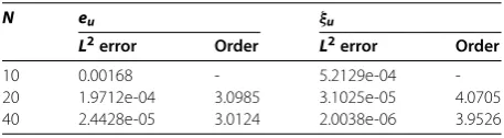
uandξuand their orders on a nonuniform mesh, which is a % random perturbation of the uniform mesh, at the final timeT= in thePpiecewise polynomial case and the final timeT= . in thePpiecewise polynomial case,
[image:14.595.179.412.562.633.2]respec-tively.
Table 1 TheL2errors and the order of the LDG method with the piecewiseP1space atT= 1
N eu ξu
L2error Order L2error Order
10 0.0283 - 0.0030
-20 0.0073 1.9485 3.7684e-04 2.9757
40 0.0018 2.0136 5.4173e-05 2.9889
80 4.7371e-04 1.9365 7.2521e-06 2.9011
Table 2 The numerical results of the LDG method with the piecewiseP2space atT= 0.1
N eu ξu
L2error Order L2error Order
10 0.00168 - 5.2129e-04
-20 1.9712e-04 3.0985 3.1025e-05 4.0705
[image:14.595.183.412.670.733.2]Table 3 The numerical results of the LDG method with the piecewiseP1space at the final timeT= 1
N eu ξu
L2error Order L2error Order
10 0.0337 - 0.0057
-20 0.0071 2.2469 7.9057e-04 2.8560
40 0.0018 2.0580 8.4326e-05 2.6283
80 4.6624e-04 1.9272 1.0537e-05 3.0005
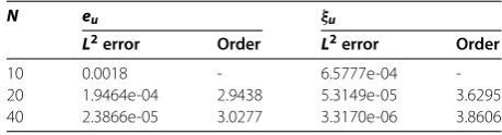
Table 4 The numerical results of the LDG method with the piecewiseP2space at the final timeT= 0.5
N eu ξu
L2error Order L2error Order
10 0.0018 - 6.5777e-04
-20 1.9464e-04 2.9438 5.3149e-05 3.6295
40 2.3866e-05 3.0277 3.3170e-06 3.8606
4.2 Example 2
We take the equation
ut+
.ux= .uxx+ .exp(–t)sin(x), x∈[–π,π],
u(x, ) =sin(x),
(.)
of which the flux function changes its sign on the computational domain. Hence, we use the Godunov flux in this example. The numerical results on the nonuniform mesh, which is a % random perturbation of the uniform mesh, are presented by Table and Table , which imply that the superconvergence property is still valid in the case that the flux func-tion is not sign preserving.
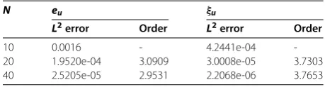
4.3 Example 3
In this example, we take an equation with a non-polynomial flux function. We have
ut+
exp(u)x
= .uxx+exp
exp(–.t)sin(x)exp(–.dt)cos(x), x∈[, π],
u(x, ) =sin(x).
(.)
The boundary condition is a periodic boundary condition. The mesh is also a % random perturbation of the uniform mesh. It results from Table and Table that the supercon-vergence property is true for a strong nonlinear flux function.
5 Conclusion
[image:15.595.181.411.222.284.2]Table 5 The numerical results of the LDG method with the piecewiseP1at the final timeT= 1
N eu ξu
L2error Order L2error Order
10 0.0252 - 0.0031
-20 0.0072 1.8027 4.3012e-04 2.8375
40 0.0018 2.0197 5.2154e-05 3.2029
80 4.4483e-04 2.0049 7.0841e-06 2.8801
Table 6 The numerical results of the LDG method with the piecewiseP2at the final timeT= 1
N eu ξu
L2error Order L2error Order
10 0.0016 - 4.2441e-04
-20 1.9520e-04 3.0909 3.0008e-05 3.7303
40 2.5205e-05 2.9531 2.2068e-06 3.7653
Future work includes the study of superconvergence of the LDG method for the nonlin-ear equations with high-order spatial derivatives in -D. The superconvergence properties of general monotone numerical flux will also be considered.
Appendix
In the appendix, we will give the proof of Lemma , which is the estimate of(eu)t.
Proof We begin by estimating(ξu)t(·, ). We deduce from (.) and (.) that
–H+jξq(·, ),vh
= –H–jξu(·, ),vh
=
Ij
eq(·, )vhdx. (A.)
Whent= , (.a) actually holds. Ifvh= (ξu)t, then we have
(ξu)t(·, )= –
(ηu)t(ξu)tdx–K
u, (ξu)t
+Kuh, (ξu)t
+
eq(ξu)tdx. (A.)
If assumption (.) holds true, we employ Lemma , the Cauchy-Schwarz inequality and estimate (.) to obtain
(ξu)t(·, )≤Chk+. (A.)
Differentiating (.a)-(.b) with respect oft, we get
(eu)ttvhdx=N L(u,uh,vh) –H+
(ξq)t,vh
, (A.a)
(eq)twhdx= –H–
(ξu)t,wh
[image:16.595.182.412.210.272.2]
where
N L(u,uh,vh) = N
j=
Ij
∂t
f(u) –f(uh)
(vh)xdx–∂t
f(u) –fu–hv–hj+/
+∂t
f(u) –fuh–v+hj–/.
Substituting (vh,wh) = ((ξu)t, (ξq)t) into (A.a)-(A.b) and applying property (.) gives
d dt(ξu)t
+(ξq)t
≤N Lu,uh, (ξu)t+
(ηu)tt(ξu)tdx
+
(ηq)t(ξq)tdx
. (A.)
We now turn to an estimate of|N L(u,uh, (ξu)t)|. The process is similar to Lemma , except for the fact that we use the second-order Taylor expansion, whose remainder is of the integral form, to deal with∂t(f(u) –f(uh)). We have
∂tf(u) –f(uh)
=∂tf(u)ηu+f(u)(ηu)t+∂tf(u)ξu
+f(u)(ξu)t–∂tIR(eu)–IReu(eu)t
=θ+θ+· · ·+θ,
∂tf(u) –fu–h=∂tf(u)ηu–+f(u)ηu–t+∂tf(u)ξu–
+f(u)ξu– t–∂tIR
e–u–IRe –ue–ut
=σ+σ+· · ·+σ,
where
IR=
( –β)fβu+ ( –β)uh
dβ,
IR=
( –β˜)fβ˜u+ ( –β˜)u–hdβ˜.
Then we set
N L
u,uh, (ξu)t=
i=
N
j=
Ij
θi
(ξu)t
xdx–σi(ξu)
–
tj+/+σi(ξu) +
tj–/
=|+++++|.
We are now ready to estimate each part:
• Noting the properties of the Gauss-Radau projection, we have
Then ||= N j= Ij
∂tf(u) –∂tf(uj)
ηu
(ξu)t
xdx
≤Cηu(ξu)t
≤Chk++C(ξu)t. (A.)
• If we do what we did in (A.) and (A.), we obtain
|| ≤Chk++C(ξu)t
. (A.)
• Dividing the integration into two parts gives
||= N j= Ij
∂tf(u) –∂tf(uj–/)
ξu
(ξu)t
xdx
–∂tf(uj+/) –∂tf(uj–/)
ξu–ξu–tj+/
+∂tf(uj–/)
Ij
ξu
(ξu)t
xdx–ξ
–
u
ξu–tj+/+ξu–ξu+tj–/
≤Chξu ·(ξu)t
x+Chξu∂(ξu)t∂+Ceq ·(ξu)t
≤Chk+(ξu)t
≤Chk++C(ξu)t. (A.)
In the second inequality, we use the Cauchy-Schwarz inequality. Using properties (.a) and (.b), we get the final step.
• Similar to the process of (A.), we obtain
|| ≤ N j= Ij
f(u) –f(uj–/)
(ξu)t
(ξu)t
xdx+f (u
j–/)
Ij
(eq)t(ξu)tdx
+f(uj–/) –f(uj+/)
ξu–tj+/
≤C(ξu)t
+ (ξq)t
+Chk+. (A.)
• If we do what we did for the estimate of||, we obtain
|| ≤Ch–eu∞eu(ξu)t ≤Chkeu∞(ξu)t
≤Chk++h–eu∞(ξu)t
, (A.)
|| ≤Ch–eu∞(eu)t(ξu)t
≤Chkeu∞(ξu)t+Ch–eu∞(ξu)t
≤Chk++Ch–eu∞+h–eu∞(ξu)t
Hence, we get
d dt(ξu)t
+(ξq)t
≤Chk++C +h–eu∞+ h–eu∞(ξu)t
. (A.)
Following estimate (.), Gronwall’s inequality and the triangle inequality, we complete
the proof.
Acknowledgements
The first author is supported by the Department of Education, Heilongjiang Province (12541133).
Competing interests
Both authors declare that they have no competing interests.
Authors’ contributions
The authors have participated in the sequence alignment and drafted the manuscript. They have approved the final manuscript.
Publisher’s Note
Springer Nature remains neutral with regard to jurisdictional claims in published maps and institutional affiliations.
Received: 31 March 2017 Accepted: 27 August 2017 References
1. Wang, C, Ding, J, Han, STW: High order numerical simulation of detonation wave propagation through complex obstacles with the inverse Lax-Wendroff treatment. Commun. Comput. Phys.18(5), 1264-1281 (2015)
2. Wang, C, Dong, XZ, Shu, CW: Parallel adaptive mesh refinement method based on WENO finite difference scheme for the simulation of multi-dimensional detonation. J. Comput. Phys.298, 161-175 (2015)
3. Wang, C, Zhang, X, Shu, CW, Ning, J: Robust high order discontinuous Galerkin schemes for two-dimensional gaseous detonations. J. Comput. Phys.231(2), 653-665 (2012)
4. Tan, S, Wang, C, Shu, CW, Ning, J: Efficient implementation of high order inverse Lax-Wendroff boundary treatment for conservation laws. J. Comput. Phys.231(6), 2510-2527 (2012)
5. Cockburn, B, Shu, C-W: The local discontinuous Galerkin method for time-dependent convection-diffusion systems. SIAM J. Numer. Anal.35(6), 2440-2463 (1998)
6. Bassi, F, Rebay, S: A high-order accurate discontinuous finite element method for the numerical solution of the compressible Navier-Stokes equations. J. Comput. Phys.131(2), 267-279 (1997)
7. Yan, J, Shu, C-W: A local discontinuous Galerkin method for KdV type equations. SIAM J. Numer. Anal.40(2), 769-791 (2002)
8. Dong, B, Shu, C-W: Analysis of a local discontinuous Galerkin method for linear time-dependent fourth-order problems. SIAM J. Numer. Anal.47(5), 3240-3268 (2009)
9. Xu, Y, Shu, C-W: Local discontinuous Galerkin methods for three classes of nonlinear wave equations. J. Comput. Math.22(2), 250-274 (2004)
10. Xu, Y, Shu, C-W: Local discontinuous Galerkin methods for high-order time-dependent partial differential equations. Commun. Comput. Phys.7(1), 1-46 (2010)
11. Zhang, Q, Shu, C-W: Error estimates to smooth solutions of Runge-Kutta discontinuous Galerkin methods for scalar conservation laws. SIAM J. Numer. Anal.42(2), 641-666 (2004)
12. Zhang, Q, Shu, C-W: Stability analysis and a priori error estimates of the third order explicit Runge-Kutta discontinuous Galerkin method for scalar conservation laws. SIAM J. Numer. Anal.48(3), 1038-1063 (2010) 13. Wang, H, Shu, C-W, Zhang, Q: Stability analysis and error estimates of local discontinuous Galerkin methods with
implicit-explicit time-marching for nonlinear convection-diffusion problems. Appl. Math. Comput.272, 237-258 (2016)
14. Cheng, Y, Shu, C-W: Superconvergence and time evolution of discontinuous Galerkin finite element solutions. J. Comput. Phys.227(22), 9612-9627 (2008)
15. Cheng, Y, Shu, C-W: Superconvergence of discontinuous Galerkin and local discontinuous Galerkin schemes for linear hyperbolic and convection-diffusion equations in one space dimension. SIAM J. Numer. Anal.47(6), 4044-4072 (2010) 16. Hufford, C, Xing, Y: Superconvergence of the local discontinuous Galerkin method for the linearized Korteweg-de
Vries equation. J. Comput. Appl. Math.255, 441-455 (2014)
17. Meng, X, Shu, C-W, Wu, B: Superconvergence of the local discontinuous Galerkin method for linear fourth-order time-dependent problems in one space dimension. IMA J. Numer. Anal.32(4), 1294-1328 (2012)
18. Yang, Y, Shu, C-W: Analysis of optimal superconvergence of discontinuous Galerkin method for linear hyperbolic equations. SIAM J. Numer. Anal.50(6), 3110-3133 (2012)
19. Yang, Y, Shu, C: Analysis of optimal superconvergence of local discontinuous Galerkin method for one-dimensional linear parabolic equations. J. Comput. Math.33, 323-340 (2015)
20. Cao, W, Zhang, Z, Zou, Q: Superconvergence of discontinuous Galerkin methods for linear hyperbolic equations. SIAM J. Numer. Anal.52(5), 2555-2573 (2014)
22. Cao, W, Shu, C-W, Yang, Y, Zhang, Z: Superconvergence of discontinuous Galerkin methods for two-dimensional hyperbolic equations. SIAM J. Numer. Anal.53(4), 1651-1671 (2015)
23. Meng, X, Shu, C-W, Zhang, Q, Wu, B: Superconvergence of discontinuous Galerkin methods for scalar nonlinear conservation laws in one space dimension. SIAM J. Numer. Anal.50(5), 2336-2356 (2012)
24. Cao, W, Li, D, Yang, Y, Zhang, Z: Superconvergence of discontinuous Galerkin methods based on upwind-biased fluxes for 1D linear hyperbolic equations. ESAIM: Math. Model. Numer. Anal.51(2), 467-486 (2017)
25. Guo, L, Yang, Y: Superconvergence of discontinuous Galerkin methods for linear hyperbolic equations with singular initial data. Int. J. Numer. Anal. Model.14(3), 342-354 (2017)