R E S E A R C H
Open Access
An effective finite element Newton
method for 2D
p-Laplace equation with
particular initial iterative function
Zhendong Luo
1*and Fei Teng
2*Correspondence: [email protected] 1School of Mathematics and Physics, North China Electric Power University, No. 2, Bei Nong Road, Changping District, Beijing, 102206, China
Full list of author information is available at the end of the article
Abstract
In this article, a functional minimum problem equivalent to thep-Laplace equation is introduced, a finite element-Newton iteration formula is established, and a
well-posed condition of iterative functions satisfied is provided. According to the well-posed condition, an effective initial iterative function is presented. Using the effective particular initial function and Newton iterations with the iterative step length equal to 1, an effective particular sequence of iterative functions is obtained. With the decreasing properties of gradient modulus of subdivision finite element, it has been proved that the function sequence converges to the solution of finite element formulation ofp-Laplace equation. Moreover, a discussion on local
convergence rate of iterative functions is provided. In summary, the iterative method based on the effective particular initial function not only makes up the shortage of the Newton algorithm, which requires an exploratory reduction in the iterative step length, but also retains the benefit of fast convergence rate, which is verified with theoretical analysis and numerical experiments.
MSC: 65N30; 35Q10
Keywords: finite element formulation; Newton method;p-Laplace equation; well-posed condition; initial iterative function
1 Introduction
Let⊂Rbe a bounded and connected domain. Consider the followingp-Laplace
equa-tion with Dirichlet boundary.
Problem I Find u such that
div(|∇u|p–∇u) =f, (x,y)∈,
u= , (x,y)∈∂, (.)
where p> ,the source term f is smooth enough to ensure validity of the following analysis and does not vanish on any nonzero measure set K(K⊂).
Thep-Laplace equation is not only a tool for researching the special theory of Sobolev spaces [], but is also an important mathematical model of many physical processes and
other applied sciences; for example, it can be used to describe a variety of nonlinear me-dia such as phase transitions in water and ice at transition temperature [], elasticity [], population models [], the non-Newtonian fluid movement in the boundary layer [], and digital image processing []. However, since the equation includes a very strong nonlinear factor, it is an important approach to solve the equation by numerical methods. A finite element method, combined with Newton iteration scheme, is one of most efficient numer-ical methods. Some posteriori error estimates for the finite element approximation of the
p-Laplace equation are developed by Carstensenet al.[, ]. Carstensen [, ] applied these posteriori error estimates to a control method of solving the equation. The control method is based on the Newton iteration. However, the Newton iteration of thep-Laplace equation is not discussed in detail in their study, which is very dependent on selection of initial iteration function and also requires an exploratory reduction in the iterative step length (the default step length is ; see []). Therefore, it is necessary to study how to select a suitable initial function. On the other hand, though the Newton algorithm has the advantage of very fast convergence rate near the solution (see []), there are many factors (for instance, the ill-posed factor) to affect the convergence of Newton iterations for thep-Laplace equation. Bermejo and Infante [] applied the Polak-Ribiere iterations to the multigrid algorithm for thep-Laplace equation instead of Newton iterations due to the difficulties in computation relating to the ill-posed coefficient matrix. In order to overcome the ill-posed problem, it is necessary to develop a well-posed condition of the iteration functions. To the best of our knowledge, a well-posed condition of the iteration functions of finite element-Newton iterations for thep-Laplace equation has not been pro-vided so far. Therefore, in this paper, we aim mainly to establish a well-posed condition of the iterative functions of finite element-Newton iterations for thep-Laplace equation and to provide theory analysis. To this end, we intend to transform the p-Laplace equation into a functional minimum problem (see Section in []) solved by Newton iterations. According to the well-posed condition, an effective particular initial function is selected, and an effective iterative function sequence is constructed. Besides, utilizing the gradient modulus and gradient direction of an element, we will discuss the factors affecting the convergence of Newton iterations.
To this end, we first introduce some special Sobolev spaces and two preparative defini-tions as follows. Let
W,p() =
v;
|∇v|p<∞
, W,p() =v∈W,p();v|∂=
with inner product and norm
(u,v) =
u·vdxdy and ∇up=
|∇u|pdxdy
/p .
In particular, we setH
() =W,() whenp= . Sincep> andis bounded, the
imbed-ding ofW,p() intoH
() is continuous (see []).
Definition For positive numbersaandb, if there exist two constantscandc(c≥c>
) independent onaandbsuch that
thenais known as the same order large (small, respectively) withb. Similarly,ais said to be high order large (small, respectively) withbif there existss> such that
cbs≤a≤cbs.
Definition For p> , a function u(x,y) is called well-posed with respect to w(x,y) (in short,u(x,y) is well-posed) if there exist two functionsc(x,y) andc(x,y) such that:
c(x,y)≥c(x,y) > ; when|∇w(x,y)| ≤,c(x,y) is at most the same order small with
|∇w(x,y)|(i.e., there is no situation of high order), andc(x,y) is at most the same order
large with /|∇w(x,y)|; when|∇w(x,y)|> ,c(x,y) is at most the same order small with
/|∇w(x,y)|, andc(x,y) is at most the same order large with|∇w(x,y)|; and
c(x,y)∇u(x,y)
p–
≤∇w(x,y)≤c(x,y)∇u(x,y)
p–
. (.)
The paper is organized as follows. In Section , a functional minimum problem equiva-lent to thep-Laplace equation is introduced, a finite element-Newton iteration formula is established, and the classical Newton algorithm is presented. In Section , we discuss the well-posed condition of iterative functions. Even though the initial function fails to satisfy the well-posed condition, after a sufficient number of Newton iterations with default step length are implemented, well-posed iterative functions can be always obtained, as will be seen in the well-posed theorem of Section . However, the iteration step number is of-ten large. So an effective particular initial iterative function that satisfies the well-posed condition should be selected in order to make the iteration step number reduced greatly. This is related to the content of Section . In Section , an effective particular iterative function sequence is provided. These functions possess some properties that the gradi-ent moduli on each subdivision finite elemgradi-ent decrease monotonically and have a certain lower boundary. By using these properties we prove that this sequence converges to the solution of finite element formulation of thep-Laplace equation and present some results about its convergence speed. In Section , considering the well-posed condition and prop-erties mentioned, we select an effective particular initial iterative function, which results in the special iterative functions involved in Section by finite element Newton itera-tions with default step length. In Section , some numerical experiments are provided for showing that some results on the convergence rate and gradient fields are consistent with theoretical conclusions.
2 A Newton algorithm for thep-Laplace equation The variational formulation of Problem I is as follows.
Problem II Find u∈W,p()such that
|∇u|p–∇u· ∇vdxdy=
fvdxdy, ∀v∈W,p(). (.)
Problem II is equivalent to solving the following functional minimum problem (see Sec-tion in []):
J(u) = min
v∈W,p()
where
J(v) :=
|∇v|pdxdy–
fvdxdy.
As far as we know, Problem II and the corresponding minimum problem have the same unique solution (see []).
This is unconstrained optimization problem with respect to scalar function, which can be solved by the Newton method (see []). According to Section in [], we can obtain the first derivative operator ofJwith respect tou:
J(u)◦δu=
|∇u|p–∇u· ∇δudxdy–
fδudxdy, ∀δu∈H(),
where the operatorJ(u) is defined on the spaceH
(), which is an inner space and more
convenient in numerical computing thanW,p(). According to continuous imbedding theory, the uniqueness of solution to Problem II inW,p() means that it also holds in
H().
Similarly, the second-derivative operator (Section in []) is written as
J(u)◦δuδu=
(p– )|∇u|p–(∇u· ∇δu)∇u+|∇u|p–∇u· ∇δu
· ∇δudxdy
for allδu,δu∈H(), By using the classical Newton algorithm we can establish the
fol-lowing Newton iteration formula. Findu–uk∈H() such that
J(uk)◦(u–uk)δu= –J(uk)◦δu, ∀δu∈H(), (.)
whereu–ukis the Newton descent direction. Furthermore, (.) can be expressed as the following equation:
(p– )|∇uk|p–∇uk· ∇(u–uk)
∇uk+|∇uk|p–∇(u–uk)
· ∇δudxdy
= –
|∇uk|p–∇uk· ∇δudxdy+
fδudxdy, ∀δu∈H(). (.)
In order to find the solution of this problem, we apply the finite element method. Let{Sh}
be a uniformly regular family of triangulation of¯ with diameters bounded byh(see []). We denote the subdivision element bye∈Shand the set of nodes byP. Let us introduce the following finite element space:
Hh=
vh∈H()∩C();vh|e∈P(e),∀e∈Sh
,
whereP(e) denotes the space of all polynomials defined on triangular elementse, and its
degree is not greater than . We set{λi}M
i=as a basis ofHh, whereMis the total number
Problem III Findδuk∈Hhsuch that
(p– )|∇uk|p–(∇uk· ∇δuk)(∇uk· ∇vh) +|∇uk|p–∇δuk· ∇vh
dxdy
= –
|∇uk|p–∇uk· ∇vhdxdy+
fvhdxdy, ∀vh∈Hh. (.)
For any nonzero measure setK⊂, the property off ensures that the iterative func-tionuk is not constant onK. Seta(uh,vh) :=
[(p– )|∇uk|p–(∇uk· ∇uh)(∇uk· ∇vh) + |∇uk|p–∇u
h· ∇vh] dxdy. Then, for anyvh∈Hhthat does not vanish on, we have the following formula:
a(vh,vh) =
(p– )|∇uk|p–(∇uk· ∇vh)+|∇uk|p–|∇vh|
dxdy
≥
|∇uk|p–|∇vh|dxdy> , ∀vh∈Hh. (.)
By the symmetry and positive definiteness ofa(·,·) there exists a uniqueuh∈Hh such that
a(uh,vh) = (f,vh), ∀vh∈Hh.
Now, we recall the classical Newton algorithm.
Step . Setk= and termination conditionε> , select an initial iterative functionu∈
Hh, and computeJ(uo).
Step . Iterative formula: apply equation (.) to findingδuk∈Hhand set iterative step lengthα:= .
Step . Setuk+:=uk+αδuk(k= , , , . . .).
Step . IfJ(uk+) <J(uk), then go to Step . Otherwise, setα:=α/ and go to Step .
Step . If [Mi=(–|∇uk+|p–∇uk+· ∇λidxdy+
fλidxdy)
]/ <ε, the algorithm
terminates, and outputuk+. Otherwise, go to Step .
Remark As will be seen in Section , the convergence speed of Newton iterative func-tions is very fast when these funcfunc-tions are near the solution to Problem II. However, the total convergence speed heavily relies on selection of an initial iterative function. So it is important to find a good initial function. On the other hand, in order to make descent, it is necessary to get an exploratory reduction in the iterative step length; see Step of the Newton algorithm. Sometimes, several attempts to shorten the step length would lead to slowing down the iteration speed. Therefore, we would give some improvements and modifications to achieve a better iteration convergence effect in the following sections.
3 Well-posed condition and well-posed theorem of iterative function 3.1 Well-posed condition
To begin with, consider the following problem: findwsuch that
–w=f, (x,y)∈,
w= , (x,y)∈∂.
Problem IV Find w∈Hhsuch that
∇w· ∇vhdxdy=
fvhdxdy, ∀vh∈Hh. (.)
Noting the relationship between the solution of Problem IV and the finite element so-lution of Problem II, denoted byu∗∈Hh, we get that, for each triangular elemente∈Sh,
∇u∗p–
∇u∗=∇w, |∇w|=∇u∗
p–
. (.)
Sincep– > , relationships of the gradient modulus of an element from (.) indicate that
u∗becomes steep ifwis gentle, and, conversely,u∗has small steepness if the gradient of
wis large.
SinceHhconsists of the piecewise continuous functions of degree , for each triangular elemente∈Shand all (x,y)∈e,|∇w(x,y)|is independent ofxandy. Iff vanishes on a
point of domain, the value of|∇w|is correspondingly very small in a small
neighbor-hood of the point. Since the domain is partitioned into small triangular elements, there exist some elements such that the values of |∇w(e)| are less than and often far less
than . As will be seen further, these triangular elements determine the convergence ef-fect of Newton iterations.
A natural idea is that the Newton initial function is selected as w, that is,u=w.
According to iterative formula (.) and (.), for each element e∈Sh, there holds the following equation:
(p– )|∇w|p–(∇w· ∇δu)∇w+|∇w|p–∇δu= –|∇w|p–∇w+∇w,
where the coefficient on the left-hand side is|∇w|p–, whereas the modulus of the second
term on the right-hand side is|∇w|. Ifp> and some elements satisfy
|∇w|p– |∇w|< ,
then there may be a situation that|∇δu|of (.) is far greater than on these elements,
which often occurs in numerical experiments involved in Section . According to the clas-sical Newton algorithm, in order to obtainJ(u) less thanJ(w), the attempts to shorten
the step length would spend many times, which will greatly affect the iteration speed. Nev-ertheless, there is no described situation for <p≤.
Generally, for a certain iterative functionuk, on each triangular elemente∈Sh, the iter-ative formula is written as
(p– )|∇w|p–(∇uk· ∇δuk)∇uk+|∇uk|p–∇δuk= –|∇uk|p–∇uk+∇w. (.)
Likewise, if some elements satisfy
|∇uk|p– |∇w|, (.)
thenδukof iterative formula (.) often has the property
The other extreme situation is that
|∇w| |∇uk|p–, (.)
whereukcannot be the finite element solution of Problem II according to (.). Therefore, both the initial function and functions of iteration should avoid the two extreme condi-tions on each elemente∈Sh, (.) and (.). This means thatukshould be well posed with respect tow, which is called the well-posed condition of iterative functions, that is,
c(e)∇uk(e) p–
≤∇w(e)≤c(e)∇uk(e) p–
, (.)
wherec(e) andc(e) meet the requirements of Definition .
Remark Thewintroduced plays a very important role in the content of the next
sub-section. Moreover, the elements where|∇w(e)| is far less than could be vital for the
convergence effect of Newton iterations. For better convergence effect, the initial iterative function need to be selected to satisfy the well-posed condition, which will be discussed in detail in Section .
3.2 Well-posed theorem of Newton iteration
Although an iterative function may fail to meet the well-posed condition, there always exists a certain iterative function satisfying the condition by the Newton iteration, as the following theorem says.
Theorem (Well-posed theorem) If there exists a domainτ⊂such that
∇uk(x,y) p–
∇w(x,y), (x,y)∈τ, (.)
then we can always obtain a certain k>k such that uk satisfies the well-posed condition
by the Newton iteration withα= .
Proof We only need to discuss the iteration onτ. By the description in Section ., the following estimate appears:
∇δuk(x,y), (x,y)∈τ.
Sinceuk+=uk+δukandp– > , the estimate onτyields
∇uk+(x,y)
p–
∇w(x,y), (x,y)∈τ. (.)
Thus, the terms on the left-hand side of iterative formula (.) can be approximated by
(p– )|∇uk+|p–(∇uk+· ∇δuk+)∇uk++|∇uk+|p–∇δuk+
In the same way, the terms on the right-hand side of (.) have the following estimate:
–|∇uk+|p–∇uk++∇w≈–|∇uk+|p–∇uk+.
Combining the preceding two estimates, we obtain that
∇δuk+≈–
p– ∇uk+.
Evidently, the gradient ofuk+can be expressed as
∇uk+=∇uk++∇δuk+≈
–
p– ∇uk+. Besides, we obtain that
|∇uk+|p–≈
–
p– p–
|∇uk+|p–,
which indicates that the gradient moduli of iterative functions decrease with a fixed rate. It is not until (.) fails to hold that the geometric decrease stops, that is, that there exists a certaink>ksuch thatuksatisfies
c|∇uk|p–≤ |∇w| ≤ |∇uk|p–≤C, whereCis a small constant, andcis defined by
c=
⎧ ⎨ ⎩
|∇w|/C if|∇w|< ,
/C otherwise,
which completes the proof of Theorem .
Corollary Let{λi}M
i=be a basis of finite element space Hhand set
G(uk+) =
M
i=
–
|∇uk+|p–∇uk+· ∇λidxdy+
fλidxdy
/
. (.)
Under the hypotheses of Theorem,we have the following estimate:
G(uk+)≈
–
p– p–
G(uk+). (.)
4 Convergence and its rate of an effective particular iterative function sequence
To begin with, we assume that the initial function satisfies
|∇w| ≤ |∇u|p–.
Since the finite element solution of Problem II satisfies (.), combining the previous in-equality and (.), we study a sequence of iterative functions whose gradient moduli de-crease on subdivision elementse∈Sh, that is, for eache∈Sh,
|∇uk+| ≤ |∇uk|.
We will use this function sequence to approximate the finite element solution of Prob-lem II, which is the main issue discussed in this section.
4.1 Decreasing conditions of gradient modulus
For each triangular elemente∈Sh, we introduce some useful notations: ∇w(e)· ∇uk(e) =rk(e)∇uk(e)
p
, rk(e)≥,∇uk(e) = (ξ,ξ)T. (.)
Take a unit vectorn= (–ξ,ξ)T/|∇uk(e)|and set
∇w(e)·n=rk(e)∇uk(e)
p–
, (.)
whererk
(e) may be positive or not.
Lemma For given function uk∈Hh,we have the following inequality on each triangular
element e∈Sh:
|∇w| ≤ |∇uk|p–. (.)
Ifδuk∈Hhis the solution of ProblemIIIand uk+=uk+δukand if rkand rksatisfy
rk(e)≤( –r k
(e))
p– –
–rk
(e)
p–
, ∀e∈Sh, (.)
then the gradient moduli on element e∈Shdecrease,that is,
|∇uk+| ≤ |∇uk|. (.)
Proof According to (.) and (.), the gradient ofwon a triangular elementeis denoted
by
∇w=rk(e)|∇uk|p–∇uk+rk(e)|∇uk|p–n, (.)
where ≤rk(e)≤ and|rk(e)| ≤. By condition (.) we have
On the elemente, taking the scalar product of (.) with ∇uk, we get |∇uk|p–∇uk· ∇δuk= –
p– |∇uk|
p–|∇uk|+
p– ∇uk· ∇w =–( –r
k
(e))
p– |∇uk|
p. (.)
Evidently, (.) means that
∇uk· ∇δuk=
–( –rk(e))
p– |∇uk|
. (.)
Likewise, taking the scalar product of (.) withn, we have
|∇uk|p–∇δuk·n=∇w·n=rk(e)|∇uk|p–
and
∇δuk·n=rk(e)|∇uk|. (.)
Due to (.) and (.),∇δukis written as
∇δuk= – –rk(e)
p– ∇uk+r k
(e)|∇uk|n. (.)
Taking the scalar product of (.) with∇δukyields |∇uk|p–|∇δuk|
= ( –p)|∇uk|p–(∇uk· ∇δuk)–|∇uk|p–∇uk· ∇δuk+∇w· ∇δuk = ( –p)|∇uk|p–(∇uk· ∇δuk)+
rk(e) – |∇uk|p–|∇uk|∇uk· ∇δuk
+rk(e)|∇uk|p–n· ∇δuk. (.) We consider the following equation:
|∇uk|p–|∇uk+|–|∇uk|
=|∇uk|p–|∇uk+∇δuk|–|∇uk|
= |∇uk|p–∇uk· ∇δuk+|∇uk|p–|∇δuk|. (.)
Combining (.)-(. ) with (.) yields the equation
|∇uk|p–|∇u
k+|–|∇uk|
=(r k
(e) – )
p– |∇uk|
p–(p– )( –rk(e))
(p– ) |∇uk|
p
+( –r k
(e))
p– |∇uk| p+rk
(e)
|∇uk|p
=
(rk
(e) – )
p– +
–rk
(e)
p–
+rk(e)
Condition (.) results in
(rk
(e) – )
p– +
–rk
(e)
p–
+rk(e)≤.
Therefore, (.) is not greater than zero, which means
|∇uk+|–|∇uk|≤,
that is,
|∇uk+| ≤ |∇uk|,
which completes the proof of Lemma .
Remark Lemma indicates that in order to make the gradient modulus of the next iterative functionuk+ less than that of uk, the projection of ∇w onto the orthogonal
component of∇ukneeds to be small enough. Furthermore, this ensures small projection of∇δuk onto orthogonal component of∇wsuch that the direction of gradient field of
uk+ is almost consistent with that ofw. This consistency is very important since the
direction of the gradient ofu∗is the same as that ofw, that is, the result of (.). As will
seen inthe next subsection, the decreasing of the gradient modulus on an elemente∈Sh is an important precondition for convergence of the iterative functions.
4.2 Convergence analysis
In order to derive the convergence of the effective particular iterative functions, we first introduce the following Lemma corresponding to Lemma .
Lemma For uk∈Hhandδuk∈Hh,let uk+=uk+δuk,and let q be conjugate of p,that
is, /p+ /q= .If uk(k= , , . . .)satisfy the requirements of Lemmaand if w∈W,p()
and u∈H(),then we have
|∇uk|pdxdy≤C, k= , , . . . , (.)
and
|∇uk|p–∇(uk+–uk)dxdy→ (k→ ∞), (.)
where C in this context indicates a positive constant that is possibly different at different occurrences.
Proof Takingvh=uk+–ukin (.) of Problem III yields that
(p– )|∇uk|p–∇uk· ∇(uk+–uk)dxdy+
|∇uk|p–∇(uk+–uk)dxdy
+
|∇uk|p–∇uk· ∇(uk+–uk) dxdy=
According to the decreasing result of Lemma , the third term on the left-hand side of (.) yields that
|∇uk|p–∇uk· ∇(uk+–uk) dxdy
=
|∇uk|p–|∇uk+|–|∇uk|–∇(uk+–uk)
dxdy
=
|∇uk|p–|∇uk+|dxdy
–
|∇uk|pdxdy–
|∇uk|p–∇(uk+–uk)dxdy
≥
|∇uk+|pdxdy
–
|∇uk|pdxdy–
|∇uk|p–∇(uk+–uk)dxdy. (.)
Combining (.) with (.) yields the following estimate:
|∇uk+|pdxdy–
|∇uk|pdxdy+
|∇uk|p–∇(uk+–uk)
dxdy
≤
∇w· ∇(uk+–uk) dxdy.
(.)
Summing (.) fromk= , , . . . ,N– and using the Young and Cauchy inequalities, we obtain that
|∇uN|pdxdy–
|∇u|pdxdy+
N– k=
|∇uk|p–∇(uk+–uk)dxdy
≤
∇w· ∇uNdxdy–
∇w· ∇udxdy
≤ ∇w,q,∇uN,p,–
∇w· ∇udxdy
≤
q
|∇w|qdxdy+
p
|∇uN|pdxdy–
∇w· ∇udxdy. (.)
Furthermore, (.) can be written as
– p
|∇uN|pdxdy–
|∇u|pdxdy
+ N– k=
|∇uk|p–∇(uk+–uk)dxdy
≤
q
|∇w|qdxdy–
∇w· ∇udxdy. (.)
Evidently, (.) and (.) hold, which completes the proof of Lemma .
The compact embedding theorem (see []) shows that, for two-dimensional space and
imbed-ding is compact:
W,p()→→C(¯).
The following theorem can be derived from this compact embedding result.
Theorem Letη∈P denote the node of Sh,and let {λi}M
i= be a basis of Hh.Under the
hypotheses of Lemma,there exits a uniqueu¯ ∈Hh such that the iterative functions uk
converge tou in the following sense¯ :
sup
η∈P
uk(η) –u¯(η)→ (k→ ∞), (.)
lim
k→∞
|∇uk|p–∇uk· ∇λidxdy=
|∇ ¯u|p–∇ ¯u· ∇λidxdy, i= , , . . . ,M. (.)
Proof Since (.) holds, due to the compact embedding theorem, (.) is easily derived, and alsouk
W
→ ¯uinW,p(), that is,
lim
k→∞g,uk=g,u¯, ∀g∈
W,p(), (.)
where (W,p())is the dual space ofW,p(). Let us introduce the space
X=|∇u|p–∇u;u∈W,p().
We note thatXis isomorphic toW,p() with the one-to-one operator
A:X→W,p(), A◦|∇u|p–∇u=u,
and its corresponding conjugate operator
A∗:W,p()→X
satisfies
g,A◦|∇u|p–∇u=A∗◦g,|∇u|p–∇u, ∀g∈W,p(). (.)
Evidently, by (.),X→→L(). For a given triangulationSh of, the basis functions of the finite element spaceHhsatisfy
sup
e∈Sh
∇λi(e)≤C, i= , , . . . ,M, (.)
which indicates that∇λi∈L∞() (i= , , . . . ,M). Due to the Riesz representation theo-rem (see []), for each∇λi, there exists a uniqueϕi∈(L())such that
∇λi,|∇uk|p–∇uk
=ϕi,|∇uk|p–∇uk
and
∇λi,|∇ ¯u|p–∇ ¯u=ϕi,|∇ ¯u|p–∇ ¯u.
Since (L())⊂X, for eachϕ
imentioned, there exists a uniquegi∈(W,p())such that
ϕi=A∗◦gi. From (.) and (.) we derive (.) by the limitation
lim
k→∞
∇λi,|∇uk|p–∇uh
= lim
k→∞
A∗◦gi,|∇uk|p–∇uk
= lim
k→∞
gi,A◦ |∇uk|p–∇uk
= lim
k→∞gi,uk=gi,u¯=
∇λi,|∇ ¯u|p–∇ ¯u
.
Thus, the proof of Theorem is completed.
Thoughukconverges tou¯by Theorem , it is still not clear whether or notu¯represents the finite element solution of Problem II. This question will be answered by Theorem . To this end, it is necessary to introduce the following lemma.
Lemma For vectorsa∈Randb∈R,there exists a constant c
> independent ofa
andbsuch that c|a–b|p≤
|a|p–a–|b|p–b·(a–b).
Theorem Under the hypotheses of Lemma,letu¯∈Hh be the convergence function of
uk,and u∗∈Hhbe the finite element solution of ProblemII.For each nodeη∈P and each
element e∈Sh,we have
¯
u(η) =u∗(η), ∇ ¯u(e) =∇u∗(e).
Proof Takingvh=λiin (.), by (.) and the Cauchy inequality we get
–|∇uk|p–∇uk+∇w
· ∇λidxdy
=
(p– )|∇uk|p–∇uk· ∇(uk+–∇uk)(∇uk· ∇λi)
+|∇uk|p–∇(uk+–uk)· ∇λi
dxdy
≤C
(p– )|∇uk|p–∇(uk+–uk)dxdy
≤C
|∇uk|p–dx
/
|∇uk|p–∇(uk+–uk)
dxdy
/
. (.)
Since∇uk,p–,≤ ∇uk,p,(see []) and∇uk,p,is bounded, (.) can be written as
–|∇uk|p–∇uk+∇w
·∇λidxdy
≤C
|∇uk|p–∇(uk+–uk)
Summing (.) fork= , , , . . . ,N– and using (.), we obtain that
∞
k=
–|∇uk|p–∇u
k+∇w
· ∇λidxdy
≤C,
which means that, for eachi(≤i≤M), we have the limitation
lim
k→∞
–|∇uk|p–∇uk+∇w
· ∇λidxdy= .
By (.) we observe that, for eachi(≤i≤M),
|∇ ¯u|p–∇ ¯u· ∇λidxdy=
∇w· ∇λidxdy.
Since{λi}Mi=is a basis of the finite element spaceHh, then for anyvh∈Hh, we have
|∇ ¯u|p–∇ ¯u· ∇vhdxdy=
∇w· ∇vhdxdy. (.)
On the other hand,u∗∈Hhis the unique finite element solution of Problem II such that
∇u∗p–∇u∗· ∇vhdxdy=
∇w· ∇vhdxdy. (.)
Owing to Lemma , subtracting (.) and (.) and takingvh=u¯–u∗yield that
c
∇
u∗–u¯pdxdy≤
∇u∗p–∇u∗–|∇ ¯u|p–∇ ¯u∇u∗–u¯dxdy= ,
wherec> . Evidently, we have
¯
u(η) =u∗(η), η∈P; ∇ ¯u(e) =∇u∗(e), e∈Sh.
Thus, the proof of Theorem is completed.
Remark Theorem shows that the gradient ofukis just weakly convergent in the sense of (.). For a stronger convergence, the further discussion will be involved in the study of convergence rate of iterative functions in the next subsection.
4.3 Convergence rate of iterative functions near the solution
To the best of our knowledge, Newton algorithms of algebraic equations have local quadratic convergence rate (see []). Among the usual optimization algorithms, such as the direct decent method and conjugate gradient method, the convergence rate of New-ton iterations near the solution is the fastest (see []). Whether or not it also works for
p-Laplace equation will be studied in this subsection.
Theorem (Local convergence rate theorem) Assume that u∗∈Hhis the solution of
Prob-lemIIsuch that
Let uk–,uk,and uk+ (k= , , . . .)be iterative functions by Newton iteration withα=
satisfying
μu∗,uk,uk–
:= sup
t∈[,],e∈Sh
|( –
t)∇u∗(e) +t∇uk(e)|p–
|∇uk–(e)|(p–)/|∇uk(e)|(p–)/
≤d, (.)
where d> is constant.Then,we have the estimate
|∇uk|p–∇uk+–u∗
dxdy
/
≤dC(p)
|∇uk–|p–∇
u∗–uk
dxdy
/
, (.)
where C(p)is a positive number that depends only on p.
Proof First, we consider the third derivative of operatorJ(u) as follows:
J(u)◦δuδuδu=
(p– )(p– )|∇u|p–(∇u· ∇δu)(∇u· ∇δu)∇u
+ (p– )|∇u|p–(∇δ
u· ∇δu)∇u
+ (p– )|∇u|p–(∇u· ∇δu)∇δu
+ (p– )|∇u|p–(∇u· ∇δu)∇δu
· ∇δudxdy
≤C(p)
|∇u|p–|∇δu||∇δu||∇δu|dxdy. (.)
From (.), the Newton iterative formula (.), and (.), according to the Taylor expan-sion with respect to a function and (.), we derive the estimate
|∇uk|p–∇(uk+–uk)
dxdy<auk+–u∗,uk+–u∗
=J(uk)◦uk+–u∗
uk+–u∗
=J(uk)◦
uk+–uk+uk–u∗
uk+–u∗
=Ju∗+J(uk)◦(uk+–uk) –J(uk)◦
u∗–uk
uk+–u∗
=Ju∗–J(uk) –J(uk)◦
u∗–uk
uk+–u∗
=
J( –t)u∗+tuk
◦u∗–uk
u∗–uk
uk+–u∗
( –t) dt
≤C(p)
( –t)∇u∗+t∇ukp–∇
u∗–uk∇
uk+–u∗dxdy
( –t) dt,
where C(p) in this context indicates a positive constant that only depends onpand is possibly different at different occurrences. For convenience, we set
ρt,u∗,uk,uk–
:= |( –t)∇u
∗(e) +t∇uk(e)|p–
By using (.) and the estimate described we have
|∇uk|p–∇uk+–u∗
dxdy
≤C(p)
ρt,u∗,uk,uk–
|∇uk–|(p–)/∇
u∗–uk
·|∇uk|(p–)/∇u
k+–u∗( –t) dtdxdy
≤C(p)
ρt,u∗,uk,uk–
|∇uk–|p–∇
u∗–uk
dxdy
/
·
|∇uk|p–∇uk+–u∗dxdy /
( –t) dt
≤C(p)μu∗,uk,uk–
|∇uk–|p–∇
u∗–uk
dxdy
/
·
|∇uk|p–∇uk+–u∗dxdy /
.
Evidently, (.) is an immediate consequence of (.) and the last estimate. The proof
of Theorem is complete.
Corollary Under the assumptions of Theorem,if ukand uk–satisfy
sup
e∈Sh
|∇u∗(e) –∇uk(e)|
|∇uk–(e)|
≤ β
dC(p), β< ,
then we have the inequality
|∇uk|p–∇uk+–u∗dxdy≤β
|∇uk–|p–∇
uk–u∗dxdy,
which indicates that
|∇uk|p–∇uk+–u∗dxdy→ (k→ ∞). (.)
Remark In the description of local convergence rate theorem, it is significant to intro-duce the definition ofμ, which relies on the relationship of the solutionu∗and iterative functionsukanduk–. More precisely, the relationship is represented by the ratio ofu∗,
uk, anduk–in the gradient modulus on an elemente∈Shwhose powers satisfy
p– = (p– )/ + (p– )/.
On the other hand, the boundedness ofμis similar to the well-posed condition foru∗,uk, anduk–such that there is no situation of high order among them. Moreover, it infers that
the iterative functionsukanduk–are in a neighborhood of the solutionu∗. This is the
the case of algebraic equations, whereas the power of|∇uk–|p–on the right-hand side is
lower than that of the term|∇uk|p–on the left-hand side. Such changes in powers mean
that the iterative functions approximate the solution more and more quickly.
Remark Corollary is a result on the stronger convergence of the gradient, compared with (.) in Theorem . However, due to the description of (.), it is different from the strong convergence inH
() orW ,p
(), which is related to the value of|∇uk|p–on
each elemente∈Shand consistent with the statement of (.) in Lemma . 5 An effective particular initial iterative function
To begin with, we introduce the particular problem
–∇ ·(|∇w|∇φ) =f, (x,y)∈,
φ= , (x,y)∈∂,
whose finite element formulation is as follows.
Problem V Findφ∈Hhsuch that
|∇w|∇φ· ∇vhdxdy=
∇w· ∇vhdxdy, ∀vh∈Hh. (.)
Evidently,on each element e∈Sh,the solutionφsatisfies
∇φ= ∇w |∇w|
, |∇φ|= . (.)
Thus,a particular initial iterative function is
u=φ+w, (.)
which satisfies the following inequality on each element e∈Sh:
|∇w| ≤ |∇u|p–. (.)
According to the theory of elliptic equations (see []), there exists a constantC> such that, on each elemente∈Sh,
∇w(e)≤C, ∇u(e)≤C+ .
Therefore, we takec(e) = +Cand
c(e) =
|∇w(e)|/( +C)p– if |∇w(e)|< ,
/( +C)p– otherwise,
such thatuis well posed. For the particular initial function, (.) plays a very important
Lemma Take the initial function udefined as in(.)and set uk∈Hhas the iterative
function by Newton formula(.)with step lengthα= .For any integer k≥and trian-gular element e∈Sh,we have the following inequalities:
|∇w| ≤ |∇uk|p–, (.)
|∇uk+| ≤ |∇uk|. (.)
Proof We use mathematical induction. First, we study the casek= . According to (.), (.), and (.), for each elemente∈Sh, we have
r(e) = . (.)
Sinceδu∈Hhis the solution of (.), due to (.) and (.),uis characterized by
∇u=∇u+∇δu=
p– +r (e)
p– |∇u| p–∇u
,
which indicatesuandwhave the same direction of the gradient field such thatu
satis-fiesr
(e) = . Therefore, fork= , Lemma shows that, on each elemente∈Sh, we have |∇u| ≤ |∇u|. Furthermore, from (.), (.), and (.) we get the following equations
on each triangular elemente∈Sh:
|∇w|=|∇u|p–r(e), |∇u|p–=|∇u|p–
p– +r (e)
p– p–
.
In order to study the relationship of these two equations, we introduce the function
g(x) =x– – ( –x)/(p– )p–, x∈[, ]. (.)
Sinceg() = andg(x) = – [ – ( –x)/(p– )]p–≥, it suffices to prove thatg(x)≤,
which means thatusatisfies (.).
Assuming thatuksatisfies
rk(e) = , (.)
we consider
uk+=uk+δuk.
Likewise, from the iterative formula (.), it follows thatrk+(e) = . Applying the method in the casek= to the general situation mentioned before, we obtain thatuk+satisfies
|∇w| ≤ |∇uk+|p–, ∇uk+| ≤ |∇uk,
Theorem Taking the initial function uas in(.)and setting uk∈Hh as the iterative
function by Newton formula (.)with step lengthα= ,then uk converges to the finite
element solution of ProblemII.
Remark As described before, in order to achieve the descent effect, the classical Newton algorithm needs a few attempts to shorten the iterative step length, whereas the particular initial function introduced in this section ensures the step length equal to . Besides, it is proved that the iterative functions based on the initial function converge to the solution for thep-Laplace equation, and the result of convergence rate theorem also holds. On the other hand, since the decreasing properties and existence of nontrivial lower boundary, these iterative functions are all well posed, whereas the well-posed theorem in Section . cannot guarantee that the subsequent functions of iteration are always well posed. In fact, this is attributed to the absence of nontrivial lower bound of gradient modulus in a well-posed theorem.
6 Some numerical experiments
In this section, we present some experiments of the Newton method to solve thep-Laplace equation based on two different initial iterative functions so as to validate the conclusion of theoretical analysis in the preceding section. To begin with, we takep= , the two-dimensional domain
=(x,y)∈R;x+y< ,
and the source functionf defined byf(x,y) =sin(πx)cos(πy).
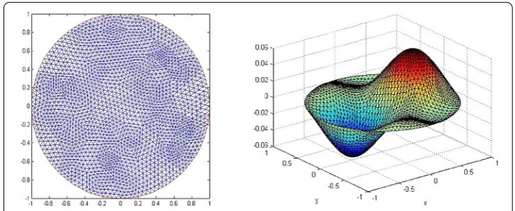
We divide the domain¯ into small triangular elements, which leads to a uniformly reg-ular triangulationShwithh≤.. The triangulation is depicted graphically on the left-hand side of Figure .
First, we consider the solutionwof Problem IV as the initial function. From the
right-hand side of Figure , the solution is characterized by a gentle and smooth shape at the peaks and troughs. According to the Newton iteration with stepα= , we obtain the nu-merical iteration functionu, depicted on the left-hand side of Figure . Evidently,uis
[image:20.595.115.479.552.701.2]not well posed: its value can reach± in some region of space owing to the large gra-dient modulus of this area. Continuing the Newton iteration with step length equal to ,
Figure 2 The left-hand side figure depicts functionu1of the first iteration; the right-hand side one is a figure of functionu29of the 29th iteration.
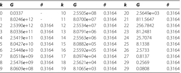
Table 1 The data record the case of 29 iterations withw0as the initial function and step
length equal to 1, wherekis the iteration number,Gis defined by (3.9), and the rateθ denotesG(uk)/G(uk–1)
k G θ k G θ k G θ
0 0.0337 - 10 2.5505e+08 0.3164 20 2.5649e+03 0.3164
1 8.0246e+12 - 11 8.0700e+07 0.3164 21 811.5647 0.3164
2 2.5390e+12 0.3164 12 2.5534e+07 0.3164 22 256.7842 0.3164 3 8.0336e+11 0.3164 13 8.0791e+06 0.3164 23 81.2481 0.3164 4 2.5419e+11 0.3164 14 2.5563e+06 0.3164 24 25.7074 0.3164 5 8.0427e+10 0.3164 15 8.0882e+05 0.3164 25 8.1338 0.3164 6 2.5448e+10 0.3164 16 2.5592e+05 0.3164 26 2.5733 0.3164 7 8.0518e+09 0.3164 17 8.0974e+04 0.3164 27 0.8137 0.3164 8 2.5476e+09 0.3164 18 2.5621e+04 0.3164 29 0.2569 0.3164 9 8.0609e+08 0.3164 19 8.1065e+03 0.3164 29 0.0808 0.3164
we spend times of iteration in finding the well-posed functionu, depicted on the
right-hand side of Figure .
The total iterations are recorded in Table including two parameters,Gandθ. Ac-cording to (.),G(uk) can determine whetherukapproximates the solution of Problem II. The smaller ofGmeans the more approximate solution obtained, and the decline rate of
Gis represented byθ. From Table , the largeGof previous iterations means that there exist some areas with very large gradient modulus, which can be inferred by the decline rateθ. Accurately, the numerical experiment verifies the conclusion of Corollary , which indicates thatGdeclines by the rate
– /(p– )p–= ..
Until the th iteration, the value ofθ becomes slightly small. The slight change shows that there are still some areas whose gradient has more significant impact on the overall convergence than that of other area.
According to the previous discussion, although the selection ofwas the initial
func-tion can result in a well-posed funcfunc-tion by the sufficient iterafunc-tions, the shortage of the geometric decrease is slow, and for the first iteration, the value ofGcan reach , likely
to cause data overflow. A conclusion can be drawn thatw is not suitable as the initial
[image:21.595.153.444.318.436.2]Figure 3 The left-hand side figure depicts the initial functionu0denoted by (5.3); the right-hand side shows the functionu8of the 8th iteration.
Table 2 The initial function is denoted by (5.3), andk,G, andθhave the same meanings with those in Table 1
k G θ k G θ
1 0.2535 0.3101 5 9.5231e–04 0.1831 2 0.0757 0.2986 6 7.9119e–05 0.0831 3 0.0210 0.2774 7 1.3964e–06 0.0176 4 0.0052 0.2476 8 7.5035e–10 5.3735e–04
on the left-hand side of Figure . According to theoretical analysis in Sections and , the particular initial function can lead to a particular sequence of iterative function with the decreasing properties of gradient modulus on each elemente, it is further proved to converge to the solution forp-Laplace equation. The numerical experiments show that we need only iterations to achieve a better result, depicted on the right-hand side of Figure and recorded in Table . Compared withw, the shape ofuat the peaks and troughs
be-come steep and sharp. As seen by the Table ,Gbecome very small after iterations, and the rateθ indicates that the decline is gradually accelerated owing to the nice selection of initial function.
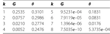
Due to the study in Remark of Section , the direction of the gradient on each ele-menteis an important factor in affecting the convergence, which is taken into account in the selection of initial function in Section . Thus, Figure shows the gradient fields ofuandw, whose directions are very similar. On the other hand, we can apply (.) to
determine whetheruapproximates the solution of Problem II, mainly by comparing the
gradient field ofwwith the vector field of|∇u|p–∇u, depicted in Figure . As seen in
Figure , the directions and lengths of arrows in the left- and right-hand side figures are almost identical, which means thatuis regarded as the approximate solution of
Prob-lem II.
7 Conclusions
Figure 4 The gradient fields ofw0andu0are showed, depicted on the left- and right-hand side, respectively.
Figure 5 The left-hand side figure depicts the gradient field ofw0; the right-hand one depicts the vector field of|∇u8|3∇u8.
In order to find a suitable initial function, the well-posed condition of the iterative func-tion is put forward, which can guarantee the absence of singularity in the iterafunc-tions. Fur-thermore, according to the well-condition theorem, we know that well-posed iterative functions always exist, except the statement that the subsequent functions of iteration with step length are all well posed, which means that despite the preceding well-posed func-tions, a subsequent function may be not well posed. This may lead to the result that the properties of iterative functions change back and forth between the well-posed and non-well-posed states. After studies, it is attributed to the absence of nontrivial lower bound of the gradient modulus. Considering the analysis described, we select a particular initial iterative function (.). By the Newton iteration with step length , the particular initial function results in a particular sequence of iterative functions with the decreasing prop-erties of the gradient modulus of a subdivision element, and it is proved to converge to the solution of finite element formulation of thep-Laplace equation in Section . Moreover, the local convergence rate shows that the convergence rate is very fast, further validated by the numerical experiments in Section .
effect is achieved and verified by the numerical experiments in Section . Evidently, for the iterative method based on the particular initial function, it is not necessary to change the iterative step length. In summary, the method not only makes up the shortage of the classical Newton algorithm, which requires an exploratory reduction in the iterative step length, but also retains the benefit of fast convergence rate.
Competing interests
The authors declare that they have no competing interests.
Authors’ contributions
All authors contributed equally to the writing of this paper. All authors read and approved the final manuscript.
Author details
1School of Mathematics and Physics, North China Electric Power University, No. 2, Bei Nong Road, Changping District,
Beijing, 102206, China.2School of Control and Computer Engineering, North China Electric Power University, No. 2, Bei Nong Road, Changping District, 102206, Beijing, China.
Acknowledgements
This research was supported by National Science Foundation of China grant 11271127 and 11671106.
Received: 5 October 2016 Accepted: 27 October 2016
References
1. Brezis, H: Functional Analysis, Sobolev Spaces and Partial Differential. Springer, New York (2010)
2. Fusco, G, Hale, JK: Slow-motion manifolds, dormant instability, and singular perturbations. J. Dyn. Differ. Equ.1, 75-94 (1989)
3. Alikakos, N, Bates, PW, Fusco, G: Slow motion for the Cahn-Hilliard equation in one space dimension. J. Differ. Equ.90, 81-135 (1991)
4. Oruganti, S, Shi, J, Shivaji, R: Diffusive logistic equation with constant yield harvesting. I. Steady states. Trans. Am. Math. Soc.354, 3601-3619 (2002)
5. Atkinson, C, Jones, CW: Similarity solutions in some nonlinear diffusion problems and in boundary-layer flow of a pseudoplastic fluid. Q. J. Mech. Appl. Math.27, 193-211 (1974)
6. Zhang, Y, Pu, Y, Zhou, J: Two new nonlinear PDE image in painting models. Comput. Sci. Environ. Eng. Ecoinformatics
158(5), 341-347 (2011)
7. Carstensen, C, Liu, W, Yan, N: A posteriori error estimates for finite element approximation of parabolic p-Laplacian. SIAM J. Numer. Anal.43(6), 2294-2319 (2006)
8. Liu, W, Yan, N: Some a posteriori error estimators forp-Laplacian based on residual estimation or gradient recovery. J. Sci. Comput.16(4), 435-477 (2001)
9. Carstensen, C, Klose, R: A posteriori finite element error control for thep-Laplace problem. SIAM J. Sci. Comput.25(3), 792-814 (2003)
10. Carstensen, C, Liu, W, Yan, N: A posteriori FE error control forp-Laplacian by gradient recovery in quasi-norm. Math. Comput.75(256), 1599-1616 (2006)
11. Bothmer, K: Numerical Methods for Nonlinear Elliptic Differential Equations: A Synopsis. Oxford University Press, Oxford (2010)
12. Bermejo, R, Infante, JA: A multigrid algorithm for thep-Laplacian. SIAM J. Sci. Comput.21(5), 1774-1789 (2000) 13. Ciarlet, PG: The Finite Element Method for Elliptic Problems. North-Holland, Amsterdam (1978)
14. Luo, ZD: Mixed Finite Element Methods and Applications. Science Press, Beijing (2006) (in Chinese) 15. Yuan, YX: Nonlinear Optimization Method. Science Press, Beijing (2008)