Accurate and efficient numerical solutions for elliptic obstacle problems

R E S E A R C H

Open Access

Accurate and efficient numerical solutions

for elliptic obstacle problems

Philku Lee

_{, Tai Wan Kim}

_{and Seongjai Kim}

*_{Correspondence:} leepk@sogang.ac.kr 1_{Department of Mathematics,} Sogang University, Ricci Building R1416, 35 Baekbeom-ro, Mapo-gu, Seoul, 04107, South Korea Full list of author information is available at the end of the article

Abstract

Elliptic obstacle problems are formulated to find either superharmonic solutions or minimal surfaces that lie on or over the obstacles, by incorporating inequality constraints. In order to solve such problems effectively using finite difference (FD) methods, the article investigates simple iterative algorithms based on the successive over-relaxation (SOR) method. It introduces subgrid FD methods to reduce the accuracy deterioration occurring near the free boundary when the mesh grid does not match with the free boundary. For nonlinear obstacle problems, a method of gradient-weighting is introduced to solve the problem more conveniently and efficiently. The iterative algorithm is analyzed for convergence for both linear and nonlinear obstacle problems. An effective strategy is also suggested to find the optimal relaxation parameter. It has been numerically verified that the resulting obstacle SOR iteration with the optimal parameter converges about one order faster than state-of-the-art methods and the subgrid FD methods reduce numerical errors by one order of magnitude, for most cases. Various numerical examples are given to verify the claim.

Keywords: elliptic obstacle problem; successive over-relaxation (SOR) method; gradient-weighting method; obstacle relaxation; subgrid finite difference (FD)

1 Introduction

Variational inequalities have been extensively studied as one of key issues in calculus of variations and in the applied sciences. The basic prototype of such inequalities is repre-sented by the so-called obstacle problem, in which a minimization problem is often solved. The obstacle problem is, for example, to find the equilibrium positionuof an elastic mem-brane whose boundary is held fixed, with an added constraint that the memmem-brane lies above a given obstacleϕin the interior of the domainΩ⊂Rd:

min

u

Ω

 +|∇u|_{dx, s.t.u≥ϕinΩ,u=f onΓ, (.)}

whereΓ =∂Ωdenotes the boundary ofΩandf is the fixed value ofuon the boundary. The problem is deeply related to the study of minimal surfaces and the capacity of a set in potential theory as well. Other classical applications of the obstacle problem include the study of fluid filtration in porous media, constrained heating, elasto-plasticity, optimal control, financial mathematics, and surface reconstruction [–].

The problem in (.) can be linearized in the case of small perturbations by expanding the energy functional in terms of its Taylor series and taking the first term, in which case the energy to be minimized is the standard Dirichlet energy

min

u

Ω

|∇u|dx, s.t.u≥ϕinΩ,u=f onΓ. (.)

A variational argument [] shows that, away from the contact set{x|u(x) =ϕ(x)}, the solu-tion to the obstacle problem (.) is harmonic. A similar argument (which restricts itself to variations that are positive) shows that the solution is superharmonic on the contact set. Thus both arguments imply that the solution is a superharmonic function. As a matter of fact, it follows from an application of the maximum principle that the solution to the ob-stacle problem (.) is the least superharmonic function in the set of admissible functions. The Euler-Lagrange equation for (.) reads

–u≥,

u≥ϕ,

(–u)·(u–ϕ) = ,

⎫ ⎪ ⎬ ⎪

⎭ inΩ,

u=f, onΓ.

(.)

In modern computational mathematics and engineering, the obstacle problems are not extremely difficult to solve numerically any more, as shown in numerous publications; see [–], for example. However, most of those known methods are either computationally expensive or yet to be improved for higher accuracy and efficiency of the numerical so-lution. In this article, we consider accuracy-efficiency issues and their remedies for the numerical solution of elliptic obstacle problems. This article makes the following contri-butions.

– Accuracy improvement through subgrid finite differencing of the free boundary: It can be verified either numerically or theoretically that the numerical solution easily involve a large error near the free boundary (the edges of obstacles), particularly when the grid mesh does not match with the obstacle edges. We suggest a post-processing algorithm which can reduce the error (by about a digit) by detecting accurate free boundary in subgrid level and introducing nonuniformfinite difference(FD) method. The main goal of the subgrid FD algorithm is to produce a numerical solution of a higher accuracyuh, which guaranteesuh(x)≥ϕ(x)forallpointsx∈Ω.

– Obstacle SOR: The iterative algorithm for solving the linear system of the obstacle problem is implemented based on one of simplest iterative algorithms, the successive over-relaxation (SOR) method. Convergence of the obstacle SOR method is analyzed and compared with modern sophisticated methods. We also suggest an effective way to set the optimal relaxation parameterω. Our simple obstacle SOR method with the optimal parameter performs better than state-of-the-art methods in both accuracy and efficiency.

positive constant. Thus the resulting system is easy to implement and presumably converges fast; as one can see from Section , the obstacle SOR algorithm for

nonlinear problems converges in a similar number of iterations as for linear problems. The article is organized as follows. The next section presents a brief review for state-of-the-art methods for elliptic obstacle problems focusing the one in []. Also, accuracy deterioration of the numerical solution (underestimation) is discussed by exemplifying an obstacle problem in D where the mesh grid does not match with edges of the free bound-ary. In Section , the SOR is applied for both linear and nonlinear problems and analyzed for convergence; the limits of iterates are proved to satisfy discrete obstacle problems. A method of gradient-weighting and second-order FD schemes are introduced for nonlin-ear problems. An effective strategy is suggested to find the optimal relaxation parameter. Section  introduces subgrid FD schemes near the free boundary in order to reduce accu-racy deterioration of the numerical solution. In Section , various numerical examples are included to verify the claims we just made. Section  concludes the article summarizing our experiments and findings.

2 Preliminaries

As preliminaries, we first present a brief review for state-of-the-art methods for elliptic obstacle problems and certain accuracy issues related to the free boundary.

2.1 State-of-the-art methods for elliptic obstacle problems

This subsection summarizes state-of-the-art methods for elliptic obstacle problems fo-cusing on theprimal-dual method incorporating L_{-like penalty term(PDLP) studied by}

Zossoet al.[]. Primal-dual splitting methods have a great deal of attention, particu-larly in the context of total variation (TV) minimization andL_{-type problems in image}

processing [–].

In the literature of optimization problems, one of common practices is to reformulate a constrained optimization problem for a unconstrained problem by incorporating the constraint as a penalty term. Recently, Tranet al.[] proposed the following minimization problem of aL_{-like penalty term:}

min

u

Ω

|∇u|+μ(ϕ–u)+, s.t.u|Γ =f, (.)

whereμis a Lagrange multiplier and (·)+=max(·, ). It is shown that, for sufficiently large

but finiteμ, the minimizer of the unconstrained problem (.) is also the minimizer of the original, constrained problem (.).

The PDLP [] is a hybrid method which combines primal-dual splitting algorithm and theL_{-like penalty method in (.); it can be summarized as follows.}

⎡ ⎢ ⎢ ⎢ ⎢ ⎢ ⎢ ⎢ ⎢ ⎢ ⎢ ⎢ ⎣

Initializeu_,u_,p_←.

Repeat

(a)pn+= (pn+r∇hun)/( +r),

(b)u∗=un_+r

∇h·pn+,

(c)un+_=P

ϕ(u∗), (d)un+= un+_–un_,

untilun+_–un

∞<ε,

where ∇h denotes the numerical approximation of the gradient∇, associated with the

mesh sizeh,randrare constants to be determined,pnis the dual variable representing

the gradient of the primal variable (un), andu∗is an intermediate solution. HerePϕis an obstacle projection defined by

Pϕ

u∗(x) =

⎧ ⎪ ⎪ ⎪ ⎨ ⎪ ⎪ ⎪ ⎩

f(x) if x∈Γ,

u∗(x) +rμ if x /∈Γ andu∗(x) <ϕ(x) –rμ,

ϕ(x) if x /∈Γ andϕ(x) –rμ≤u∗(x)≤ϕ(x),

u∗(x) otherwise.

(.)

The above algorithm can be implemented effectively. It follows from (.)(a) that

∇h·pn+=∇h· pn_+r

hun

 +r

, (.)

wherehis the discrete Laplacian. ThusSn+≡ ∇h·pn+can be considered as a variable

and updated in each iteration, averaging its previous iterateSnandhunas in (.). As

analyzed in [], PDLP (away from the obstacle) can be compared to either the forward Euler (explicit) scheme for discrete heat equation or a three-level time stepping method for a damped acoustic wave equation, whererrplays the role of the time-step size. PDLP

converges when

rrh ≤, (.)

wherehis the operator/induced norm of the discrete Laplacianh (= , when the

mesh sizeh= ). The authors in [] claimed that ‘[Their] results achieve state-of-the-art precision in much shorter time; the speed up is one-two orders of magnitude with respect to the method in [], and even larger compared to older methods [–].’ Thus, in this article our suggested method would be compared mainly with PDLP (the best-known method), in order to show its superiority.

2.2 Accuracy issues

The solution of obstacle problems must lie on or over the obstacle (u≥ϕ), which is also one of requirements for numerical solutions. For FD methods and finite element(FE) methods for the obstacle problem (.), for example, this requirement can easily be vi-olated when edges of the free boundary does not match with mesh grids. See Figure , where the shaded rectangle indicates the obstacle defined on one-dimensional (D) inter-val [x,x]:

ϕ(x) =

 ifx≤x<p,

 ifp≤x≤x,

(.)

Figure 1 A non-matching grid: The true solutionu(red solid curve) and the numerical solution on the non-matching grid uh(blue dashed curve).Here the obstacle is the shaded region,

which is not matching with the mesh grids{xi:xi=i·hx,i= , . . . , }. The figure shows the

true solutionu(red solid curve) and a numerical solutionuh(blue dashed curve) of the

linear obstacle problem (.) in D. The numerical solution is clearly underestimated and the magnitude of the error|uh–u|is maximized atx=p:

max

x uh(x) –u(x)=uh(p

–u(p)= x–p

x–x

, (.)

which isO(hx).

LetChdenote the numerical contact set:

Ch≡

x∈Ω_h:uh(x) =ϕ(x)

, (.)

whereΩ_his the set ofinteriorgrid points. Define an interior grid point is aneighboring pointif it is not in the contact set but one of its adjacent grid points is in the contact set. Let the set of neighboring points be called theneighboring set Nh. Then, for the example

in Figure ,Ch={x,x}andNh={x}.

The accuracy of the numerical solution uh can be improved by applying a

post-processing in which a subgrid FD method is applied at grid points in the neighboring set. For example, atx=x, –uxxcan be approximated by employing nonuniform FD schemes

over the grid points [x,x,p], given as

–uxx(x)≈



h

x

– u  +r+

u

r –

ϕ(p)

r( +r)

, (.)

wherer= (p–x)/hx∈(, ], and therefore numerical solution of –uxx=  atx=xmust

satisfy

u=

ru+ϕ(p)

 +r . (.)

Asris approaching  (i.e., (p–x) becomes smaller proportionally), the obstacle value

ϕ(p) is more weighted. On the other hand, whenr= ,ϕ(p) =uand the scheme in (.)

becomes the standard second-order FD scheme. Let the numerical solutionube obtained from

ϕ(xj)≤uj=

(ruj–+ϕ(p))/( +r) ifj= ,

(uj–+uj+)/ ifj= , , ,

(.)

whereu=  andu= . Then it is not difficult to prove thatuisexactlythe same as the

true solutionuat all grid points (except numerical rounding error), regardless of the grid sizehx.

The above example has motivated the authors to develop an effective numerical algo-rithm for elliptic obstacle problems in D which detects the neighboring set of the free boundary, determines the subgrid proportions (r’s), and updates the solution for an im-proved accuracy using subgrid FD schemes. Here the main goal is to try to guarantee

3 Obstacle relaxation methods

This section introduces and analyzes effective relaxation methods for solving (.) and its nonlinear problem as shown in (.) below.

3.1 The linear obstacle problem

We will begin with second-order approximation schemes for –u. For simplicity, we con-sider a rectangular domain inR_{,Ω= (a}

x,bx)×(ay,by). Then the following second-order

FD scheme can be formulated on the grid points:

xpq:= (xp,yq), p= , , . . . ,nx,q= , , . . . ,ny, (.)

where, for some positive integersnxandny,

xp=ax+p·hx, yq=ay+q·hy; hx= bx–ax

nx

,hy= by–ay

ny

.

Letupq=u(xp,yq). Then, at each of the interior points xpq, the five-point FD approximation

of –ureads

–hupq=

–up–,q+ upq–up+,q h

x

+–up,q–+ upq–up,q+

h

y

. (.)

Multiply both sides of (.) byh

xto have

(–hupq)hx=

 + r_xyupq–up–,q–up+,q–rxyup,q––rxyup,q+, (.)

whererxy=hx/hyandust=fstat boundary grid points (xs,yt).

Now, consider the following Jacobi iteration for simplicity. Given an initializationu, findun_{iteratively as follows.}

AlgorithmLJ

Forn= , , . . . Forq=  :ny– 

Forp=  :nx– 

(a)uJ,pq=_+_r xy(u

n–

p–,q+unp–+,q+rxyupn–,q–+rxyunp–,q+);

(b)un

pq=max(uJ,pq,ϕpq);

end end end

(.)

whereun–

st =fstat boundary grid points (xs,yt).

Note that AlgorithmLJproduces a solutionuof which the function value at a point is a

Theorem  Letu be the limit of the iterates un_{of AlgorithmL}

J.Thenu satisfies the FD discretization of(.).That is,

–hupq≥, upq≥ϕpq,

(–hupq)·(upq–ϕpq) = , ⎫ ⎪ ⎬ ⎪

⎭ (xp,yq)∈Ω



h,

ust=fst, (xs,yt)∈Γh,

(.)

whereΩ_hdenotes the set of interior grid points andΓhis the set of boundary grid points. Proof It is clear to see from AlgorithmLJthat

upq≥ϕpq for (xp,yq)∈Ωh and ust=fst for (xs,yt)∈Γh.

Letupq=ϕpqat an interior point (xp,yq). Then it follows from (.)(b) that

uJ,pq=

  + r

xy

up–,q+up+,q+rxyup,q–+rxyup,q+

≤ϕpq=upq, (.)

which implies that

≤ + r_xyupq–up–,q–up+,q–rxyup,q––rxyup,q+= (–hupq)·hx. (.)

On the other hand, letupq>ϕpqat (xp,yq). Then, sinceupq=max(uJ,pq,ϕpq), we must have

upq=uJ,pq, (.)

which implies that –hupq= . This completes the proof.

One can easily prove that the algebraic system obtained from (.) is irreducibly di-agonally dominant and symmetric positive definite. Since its off-diagonal entries are all nonpositive, the matrix must be a Stieltjes matrix and therefore an M-matrix []. Thus relaxation methods of regular splittings (such as the Jacobi, the Gauss-Seidel (GS), and the successive over-relaxation (SOR) iterations) are all convergent and their limits are the same asuand therefore satisfy (.). In this article, variants of AlgorithmLJfor the GS

and the SOR would be denoted, respectively, byLGSandLSOR(ω), whereωis an

over-relaxation parameter for the SOR,  <ω< . For example,LSOR(ω) is formulated as

AlgorithmL_SOR(ω) Forn= , , . . .

Forq=  :ny– 

Forp=  :nx– 

(a)uGS,pq=_+_r xy(u

n

p–,q+unp–+,q+rxyupn,q–+rxyunp,–q+);

(b)uSOR,pq=ω·uGS,pq+ ( –ω)·unpq–;

(c)un_pq=max(uSOR,pq,ϕpq);

end end end

(.)

whereun–

Note that the right side of (.)(a) involves updated values wherever available. When ω= , AlgorithmLSOR(ω) becomes AlgorithmLGS; that is,LSOR() =LGS.

3.2 The nonlinear obstacle problem

Applying the same arguments for the linear problem (.), the Euler-Lagrange equation for the nonlinear minimization problem (.) can be formulated as

N(u)≥,

u≥ϕ,

N(u)·(u–ϕ) = ,

⎫ ⎪ ⎬ ⎪

⎭ inΩ,

u=f, onΓ,

(.)

where

N(u) = –∇ ·

_∇

u

 +|∇u|

. (.)

Thus the solution to the nonlinear problem (.) can be considered as a minimal surface satisfying the constraint given by the obstacle functionϕ.

Since +|∇u|_{≥, the nonlinear obstacle problem (.) can equivalently be}

formu-lated as

M(u)≥,

u≥ϕ,

M(u)·(u–ϕ) = ,

⎫ ⎪ ⎬ ⎪

⎭ inΩ,

u=f, onΓ,

(.)

where

M(u) = – +|∇u|_{∇ ·}

_∇

u

 +|∇u|

. (.)

Such a method of gradient-weighting will make algebraic systems simpler and better conditioned, as to be seen below. In order to introduce effective FD schemes forM(u), we first rewriteM(u) as

M(u) = – +|∇u| 

ux

 +|∇u|

x

– +|∇u| 

uy

 +|∇u|

y

, (.)

where both ( +|∇u|₎  and (

 +|∇u|₎

 are the same as

 +|∇u|_{; however, they}

For the FD scheme at the (p,q)th pixel, we first compute second-order FD approxima-tions of +|∇u|_{at x}

p–/,q(W), xp+/,q(E), xp,q–/(S), and xp,q+/(N):

dpq,W=

 + (upq–up–,q)/hx

+ (up–,q++up,q+–up–,q––up,q–)/

h_y/,

dpq,E=dp+,q,W, dpq,S=

 + (upq–up,q–)/hy

+ (up+,q+up+,q––up–,q–up–,q–)/

h_x/,

dpq,N =dp,q+,S.

(.)

Then the directional-derivative terms at the pixel point xpqcan be approximated by

ux

 +|∇u|

x

(xpq)≈



h

x



dpq,W up–,q+



dpq,E up+,q–



dpq,W

+ 

dpq,E upq , uy

 +|∇u|

y

(xpq)≈



h

y



dpq,S up,q–+



dpq,N up,q+–



dpq,S

+ 

dpq,N

upq

.

(.)

Now, we discretize the surface element as follows:

 +|∇u| (xpq)≈

 



dpq,W

+ 

dpq,E

–

= dpq,Wdpq,E

dpq,W+dpq,E

,

 +|∇u| (xpq)≈

 



dpq,S

+ 

dpq,N

–

= dpq,Sdpq,N

dpq,S+dpq,N

,

(.)

where the right-hand sides are harmonic averages of FD approximations of +|∇u|_in

x- andy-coordinate directions, respectively. Then it follows from (.), (.), and (.) that

M(u)(xpq)·hx≈

 + r_xyupq–apq,Wup–,q–apq,Eup+,q

–r_xyapq,Sup,q––rxyapq,Nup,q+, (.)

where

apq,W=

dpq,E dpq,W+dpq,E

, apq,E=

dpq,W dpq,W+dpq,E

,

apq,S=

dpq,N dpq,S+dpq,N

, apq,N=

dpq,S dpq,S+dpq,N

.

(.)

Note thatapq,W+apq,E=apq,S+apq,N= . As for the linear problem, it is easy to prove that

the algebraic system obtained from (.) is an M-matrix.

AlgorithmNJ

Forn= , , . . . Forq=  :ny– 

Forp=  :nx– 

(a)uJ,pq=_+_r xy(a

n–

pq,Wunp––,q+anpq–,Eunp–+,q+rxyapqn–,Sunp–,q–+rxyanpq–,Nunp–,q+);

(b)un

pq=max(uJ,pq,ϕpq);

end end end

(.)

whereun–

st =fstat boundary grid points (xs,yt).

The superscript (n– ) on the coefficientsapq,D,D=W,E,S,N, indicate that they are

ob-tained using the last iterateun–_{. AlgorithmN}

Jproduces a solutionuof which the function

value at a point is aweightedaverage of four neighboring values, satisfying the constraint

u≥ϕ. One can prove the following corollary, using the same arguments introduced in the proof of Theorem .

Corollary  Letu be the limit of the iterates un_{of AlgorithmN}

J.Thenu satisfies the FD discretization of(.).That is,

Mh(u)pq≥, upq≥ϕpq,

Mh(u)pq·(upq–ϕpq) = , ⎫ ⎪ ⎬ ⎪

⎭ (xp,yq)∈Ω



h,

ust=fst, (xs,yt)∈Γh,

(.)

whereMh(u)pqdenotes the FD scheme ofM(u)(xpq)as defined in(.)with u=u.

Variants of AlgorithmNJfor the GS and the SOR can be formulated similarly as for the

linear obstacle problem; they would be denoted respectively byNGSandNSOR(ω). In

prac-tice, such symmetric coercive optimization problems, the SOR methods are much more efficient than the Jacobi and Gauss-Seidel methods. We will exploitLSOR(ω) andNSOR(ω)

for numerical comparisons with state-of-the-art methods, by setting the relaxation pa-rameterωoptimal.

3.3 The optimal relaxation parameter

ω

Consider the standard Poisson equation with a Dirichlet boundary condition

–u=g inΩ,

u=f onΓ =∂Ω,

(.)

for prescribed functionsf andg. LetΩ= [, ], for simplicity, and apply the second-order FD method for the second derivatives on a uniform grid:h=hx=hy= /(m+ ), for some

positive integer. The its algebraic system can be written as

Then the theoretically optimal relaxation parameter for the SOR method can be deter-mined as [], Section .,

ω= 

 + –ρ(TJ)

, (.)

where ρ(TJ) is the spectral radius of the iteration matrix of the Jacobi methodTJ. The

iteration matrixTJcan be explicitly presented as a block tridiagonal matrix

TJ=



tridiag(Im,Bm,Im), (.)

whereImis them-dimensional identity matrix and

B=tridiag(, , ) =

⎡ ⎢ ⎢ ⎢ ⎢ ⎢ ⎢ ⎢ ⎣

 

  

. .. ... ...

  

 

⎤ ⎥ ⎥ ⎥ ⎥ ⎥ ⎥ ⎥ ⎦

∈Rm×m_.

For such a matrixTJ, it is well known that

ρ(TJ) =  –ch, for somec> . (.)

Thus it follows from (.) and (.) that the optimal SOR parameter corresponding to the mesh sizeh,ωh, can be expressed as

ωh=



 + – ( –ch₎ =



 +√ch_–c_h≈

  +ch

, (.)

wherec=

√

c. Hence, for general mesh sizeh, the corresponding optimal SOR parame-terωhcan be found as follows.

⎧ ⎪ ⎪ ⎪ ⎨ ⎪ ⎪ ⎪ ⎩

(a) Determineωhfor a prescribed mesh sizeh=h,heuristically.

(b) Findcby solving (.) forc:

c= (/ωh– )/h.

(c) Use (.) with the abovecto determineωhfor generalh.

(.)

It is often the case that the calibration (.)(a)-(.)(b) can be carried out with a small problem,i.e., withhof a very low resolution.

4 Subgrid FD schemes for the free boundary: a post-process

This section describes subgrid FD schemes for the free boundary, focusing on the linear obstacle problem; the arguments to be presented can be applied the same way for nonlin-ear problems. Again, we assume for simplicity thath=hx=hy.

However, when the mesh grid is not matching with the free boundary, the obstacle con-straintu≥ϕmay not be satisfied at all points x∈Ω. This implies that when the mesh is not fine enough, the numerical solution can be underestimated near the free boundary, as shown in Figure  in Section .. Note that the error introduced by non-matching grids is inO(h), while the numerical truncation error is inO(h_{) for second-order FD schemes.}

That is, the underestimation is in O(h), which can be much larger than the truncation error. The strategy below can be considered as a post-processing algorithm designed in order to reduce the underestimation without introducing a mesh refinement. The post-processing algorithm consists of three steps: (a) finding the numerical contact set and the neighboring set, (b) subgrid determination of the free boundary, and (c) nonuniform FD schemes on the neighboring set.

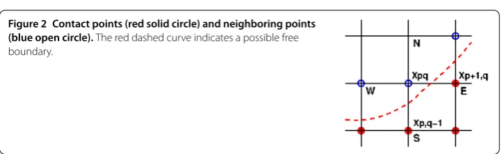
4.1 The contact set and the neighboring set

Finding the numerical contact set is an easy task. Letuandϕbe the numerical solution and the lower obstacle, respectively. Then, for example, the characteristic set of contact pointsChcan be determined as follows.

⎡ ⎢ ⎣

Ch=u–ϕ;

ifCh(xpq) > , thenCh(xpq) = ; for all points xpq; Ch=  –Ch.

(.)

As defined in Section ., an interior grid point is a neighboring point when it is not in the contact set but one of its adjacent grid points is in the contact set. Thus the neighboring points can be found more effectively as follows. Visit each point in the contact set; if any one of its four adjacent points is not in the contact set, then the non-contacting point is a neighboring point. The set of all neighboring points is the neighboring setNh.

4.2 Subgrid determination of the free boundary

Let xpq be a neighboring point with two of its adjacent points are contact points

(Ch(p+ ,q) =Ch(p,q– ) = ), as in Figure . Then we may assume that therealfree

boundary passes somewhere between the contact points and the neighboring points. We will suggest an effective strategy for the determination of the free boundary in subgrid level.

We first focus on the horizontal line segment connecting xpqand xp+,qin the east (E)

direction. Define

xE(r) = ( –r)xpq+rxp+,q, r∈[, ]. (.)

Then the corresponding linear interpolation between upqand up+,qover the line segment

is formulated as

LE(r) = ( –r)upq+rup+,q, r∈[, ]. (.)

Let

FE(r) =ϕ

xE(r)

–LE(r), r∈[, ]. (.)

Since xpqand xp+,qare a neighboring point and a contact point, respectively, we have

FE() <  and FE() = . (.)

If the free boundary passes between xpqand xp+,q, then there must existr∈(, ) such that FE(r) > . LetrEbe such that xE(rE) represents the intersection between the line segment

xE(·) and the free boundary. Then it can be approximated as follows.

rE=max

r∈(,]FE(r). (.)

The maximization problem in (.) can be solved easily (using the Newton method, for example), when the obstacle is defined as a smooth function. A more robust method can be formulated as a combination of a line search algorithm and the bisection method.

setk,k;

rE= ; Fmax= ;

fork=  :k–  % line search

ifFE(k/k) >Fmax

rE=k/k; Fmax=FE(k/k);

end end

ifrE<  % refine it through bisection rb= /k;

fork=  :k

rb=rb/;

ifFE(rE–rb) >Fmax

rE=rE–rb; Fmax=FE(rE–rb);

end

ifFE(rE+rb) >Fmax

rE=rE+rb; Fmax=FE(rE+rb);

end end

BE=ϕ(xE(rE));

end

(.)

Remarks

– The last evaluation ofϕ(and saving) is necessary for the nonuniform FD schemes on the neighboring set, which will be discussed in Section .. The quantityBEwill be

– For other directionsD(=W,S, orN), one can define corresponding difference functionsFDas shown in (.)-(.) forD=E. ThenrDcan be obtained by applying

(.) withFEbeing replaced withFD. When the adjacent pointxD()is not a contact

point, you may simply setrD= . Thus each neighboring point produces an array of

four values[rW,rE,rS,rN]and free boundary values for the directionsDwhererD< .

– Assuming that (.) has a unique solution and the obstacle is given as a smooth function, the maximum error for the detection of the free boundary using (.) is



k·

 k

h, (.)

wherehis mesh size. It has been numerically verified that the choice(k,k) = (, )

is enough for an accurate detection of the free boundary, for which the upper bound of the error becomesh/ = .h.

4.3 Nonuniform FD schemes on the neighboring set

Let xpq= (xp,yq) be a neighboring point. Thenrpq,D∈(, ] would be available for each D∈ {W,E,S,N};Bpq,Dis also available forrD< . Thus the FD scheme for –uxx(xpq) can be

formulated over three points{(xp–rpq,Whx,yq), (xp,yq), (xp+rpq,Ehx,yq)}as follows.

–uxx(xpq)≈



h

x

– upq,W

rpq,W(rpq,W+rpq,E)

+ upq

rpq,W·rpq,E

– upq,E

rpq,E(rpq,W+rpq,E)

, (.)

where

upq,W=

up–,q ifrpq,W= , Bpq,W ifrpq,W< ,

upq,E=

up+,q ifrpq,E= , Bpq,E ifrpq,E< .

Similarly, the FD scheme for –uyy(xpq) can be formulated over three points in the y

-direction{(xp,yq–rpp,Shy), (xp,yq), (xp,yq+rpp,Nhy)}:

–uyy(xpq)≈



h

y

– upq,S

rpq,S(rpq,S+rpq,N)

+ upq

rpq,S·rpq,N

– upq,N

rpq,N(rpq,S+rpq,N)

, (.)

where

upq,S=

up,q– ifrpq,S= , Bpq,S ifrpq,S< ,

upq,N=

up,q+ ifrpq,N = , Bpq,N ifrpq,N < .

Thus, the post-processing algorithm of the obstacle SOR (.),LSOR(ω), can be

formu-lated by replacing the two terms in the right side of (.) with the right sides of (.) and (.), and computinguGS,pqin (..a) correspondingly at all neighboring points.

5 Numerical experiments

Intel i-S . GHz processor. The optimal relaxation parameter is calibrated with the lowest resolution to find a constant c(.) and the constant is used for all other

cases. For a comparison purpose, we implemented a state-of-the-art method, PDLP [], and its parameters (randrin (.)) are found heuristically for cases where the

param-eters are not suggested in []. The iterations are stopped when the maximum difference of consecutive iterates becomes smaller than the toleranceε:

un_–un–

∞<ε, (.)

whereε= –mostly; Section . usesε= – for an accurate estimation of the error. For all examples, the numerical solution is initialized fromϕ(the lower obstacle) and the boundary conditionf.

u(x) =

ϕ(x) if x∈Ω

h, f(x) if x∈Γh.

(.)

5.1 Linear obstacle problems

We first consider a non-smooth obstacleϕ:Ω→RwithΩ= [, ], defined by

ϕ(x,y) =

⎧ ⎪ ⎪ ⎪ ⎨ ⎪ ⎪ ⎪ ⎩

 if|x– .|+|y– .|< ., . if (x– .)_{+ (y– .)}_{< .,}

. ify= . and . <x< .,  otherwise.

(.)

We solve the linear obstacle problem varying resolutions. The tolerance is setε= –

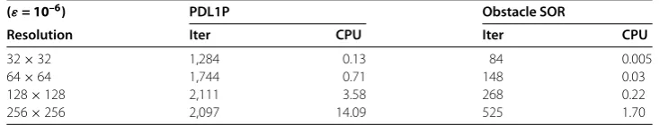
hereafter except for examples in Section .. Table  presents the number of iterations and CPU (the elapsed time, measured in second) for the linear problem of the non-smooth ob-stacle (.). One can see from the table that our suggested method requires less iterations and converges about one order faster in the computation time than the PDLP, a state-of-the-art method. We have also implemented the primal-dual hybrid gradient (PDHD) algorithm in [, , ] for obstacle problems. The PDLP turns out to be a simple adap-tation of the PDHD and their performances are about the same, particularly whenμis set large. For the resolution ×, Figure  depicts the numerical solutions of the PDLP and the obstacle SOR and their contour lines. For this example, both the PDLP and the obstacle SOR resulted in almost identical solutions.

Table 1 The number of iterations and CPU for the linear problem of the non-smooth obstacle

ϕ1(5.3)

(ε= 10–6_{) PDL1P Obstacle SOR}

Resolution Iter CPU Iter CPU

32×32 1,284 0.13 84 0.005

64×64 1,744 0.71 148 0.03

128×128 2,111 3.58 268 0.22

256×256 2,097 14.09 525 1.70

Figure 3 Solutions to the linear problem for the obstacleϕ1(5.3) at resolution 64×64. (a)The numerical solution by the PDL1P,(b)its contour plot,(c)the numerical solution by the obstacle SOR, and (d)its contour plot.

As the second example, we consider the radially symmetric obstacleϕ:Ω→Rwith

Ω= [–, ]_{defined by}

ϕ(r) =

√

 –r _ifr≤r∗_,

– otherwise, (.)

wherer∗= . . . . , the solution of

r∗ –logr∗/= . (.)

For the obstacleϕ, the analytic solution to the linear obstacle problem can be defined as

u∗(r) = √

 –r _ifr≤_r∗_,

–(r∗)_{ln(r/)/ – (r}∗₎ _otherwise, (.)

when the boundary condition is set appropriately usingu∗. See Figure , in which we give plots ofϕand the true solutionu∗.

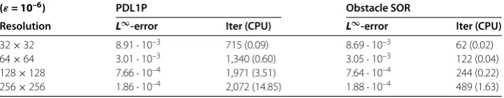
In Table , we compare performances of the PDLP and the obstacle SOR applied for the linear obstacle problem with (.). The PDLP uses the parameters suggested in [] (μ= .,r= .,r= .). As one can see from the table, our suggested method

Figure 4 The true solution to the linear problem for the obstacleϕ2(5.4) at resolution 64×64. (a)The obstacleϕ2and(b)the true solutionu∗(5.6)

Table 2 L∞-errors, the number of iterations, and the CPU for linear obstacle problem withϕ2 (5.4)

(ε= 10–6_{) PDL1P Obstacle SOR}

Resolution L∞-error Iter (CPU) L∞-error Iter (CPU)

32×32 8.91·10–3 _{715 (0.09) 8.69·10}–3 _{62 (0.02)}

64×64 3.01·10–3 _{1,340 (0.60) 3.05·10}–3 _{122 (0.04)}

128×128 7.66·10–4 _{1,971 (3.51) 7.64·10}–4 _{244 (0.22)}

256×256 1.86·10–4 _{2,072 (14.85) 1.88·10}–4 _{489 (1.63)}

The PDL1P uses the parameters suggested in [14] (μ= 0.1,r_{1 = 0.008},r_{2 = 15.625}).

by the PDLP and the obstacle SOR at the × resolution. The solutions are almost identical and the errors are nonpositive. This implies that the numerical solutions of the obstacle problem are underestimated.

As a more general obstacle problem, we consider the elastic-plastic torsion problem in []. The problem is to find the equilibrium position of the membrane between two obstaclesϕ,ψthat a forcevis acting on:

min

u

Ω

|∇u|dx–

Ω

uv dx, s.t.ψ≥u≥ϕinΩ,u=f onΓ. (.)

LetΩ= [, ]_{and the problem consist of two obstaclesϕ}

:Ω→R,ψ:Ω→Rand the

forcev:Ω→Rdefined byϕ(x,y) = –dist(x,∂Ω),ψ(x,y) = . and

v(x,y) =

⎧ ⎪ ⎨ ⎪ ⎩

 if (x,y)∈S={(x,y) :|x–y| ≤.∧x≤.}, –ey_{g(x) ifx≤ –yand (x,y) /∈S,}

ey_{g(x) ifx>  –yand (x,y) /∈S,}

(.)

where

g(x) =

⎧ ⎪ ⎪ ⎪ ⎪ ⎪ ⎪ ⎪ ⎪ ⎨ ⎪ ⎪ ⎪ ⎪ ⎪ ⎪ ⎪ ⎪ ⎩

x if ≤x≤/, ( – x) if / <x≤/, (x– /) if / <x≤/, ( – (x– /)) if / <x≤/, (x– /) if / <x≤/, ( – (x– /)) if / <x≤.

Figure 5 Numerical solutionsuhand errorsuh–u∗at the 64×64 resolution. (a)-(b)by the PDL1P and (c)-(d)by the obstacle SOR.

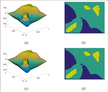
Figure 6 Elastic-plastic torsion problem. (a)The obstacles (ψ3andϕ3) and(b)the forcev.

See Figure , where the obstacles and the force are depicted.

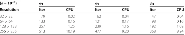
In Table , we present performances of the PDLP and the obstacle SOR applied for the elastic-plastic torsion problem (.). For the PDLP, we use the parameters suggested in [] (μ= .,r = .,r= .). As one can see from the table, our suggested

Table 3 The number of iterations and the CPU time for the elastic-plastic torsion problem (5.7)

(ε= 10–6_{) PDL1P Obstacle SOR}

Resolution Iter CPU Iter CPU

32×32 887 0.13 47 0.02

64×64 1,287 0.68 98 0.04

128×128 1,609 3.43 193 0.22

256×256 1,866 17.27 368 1.58

For the PDL1P, we use the parameters suggested in [14] (μ= 0.1,r_{1 = 0.008},r_{2 = 15.625}).

Figure 7 The numerical solutions and the contact sets for the elastic-plastic torsion problem at the 64×64 resolution. (a)-(b)by the PDL1P and(c)-(d)by the obstacle SOR.

and (d), the upper and lower contact sets are colored in yellow (brightest in gray scale) and blue (darkest in gray scale), respectively. The results produced by the two methods areapparentlythe same.

5.2 Nonlinear obstacle problems

The obstacle SOR is implemented for nonlinear obstacle problems as described in Sec-tion ..

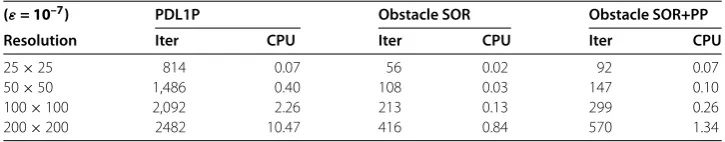
In Table , we present experiments for which the obstacle SOR is applied for nonlinear obstacle problems withϕ=ϕi,i= , , . From a comparison with linear cases presented in

Table 4 The performance of the obstacle SOR applied for nonlinear obstacle problems with

ϕ=ϕ_i,i= 1, 2, 3

(ε= 10–6_{) ϕ1 ϕ2 ϕ3}

Resolution Iter CPU Iter CPU Iter CPU

32×32 79 0.02 62 0.04 47 0.04

64×64 133 0.16 121 0.17 98 0.16

128×128 257 1.25 239 1.16 192 1.09

256×256 513 10.19 477 9.20 368 8.24

Figure 8 Nonlinear obstacle problem withϕ=ϕ1at resolution 64×64. (a)The nonlinear numerical solution and(b)its contour plot.

Figure 9 The difference between the linear solution and the nonlinear solution, at the 64×64 resolution, for the obstacle problem withϕ=ϕ1. (a)(uh,linear–uh,nonlinear) and(b)its density plot.

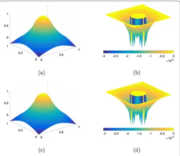
Only the apparent difference is the CPU time; an iteration of the nonlinear solver is about as six time expensive as that of the linear solver, due to the computation of coefficients as in (.). Forϕ=ϕ, the nonlinear solution is plotted in Figure . Compared with the linear

5.3 Post-processing algorithm

In Figure , one have seen that the error, the difference between the numerical solution and the analytic solution, shows its highest values near the free boundary. The larger error is due to the result of mismatch between the mesh grid and the obstacle edges. In order to eliminate the error effectively, we apply the subgrid FD schemes in Section  as a post-processing (PP) algorithm. For the examples presented in this subsection, the numerical solutions are solved as follows: (a) the problem is solved withε= –_{(pre-processing),}

(b) the free boundary is estimated with (k,k) = (, ) and subgrid FD schemes are

ap-plied at neighboring grid points as in Section , and (c) another round of iterations is applied to satisfy the toleranceε= –_.

First, we consider a step function for an one-dimensional (D) obstacle, as in Section .. LetΩ= [, ] andϕ:Ω→Rdefined by

ϕ(x) =

 if ≤x<π/,

 ifπ/≤x≤. (.)

The analytic solution to the linear problem is given as

u,true(x) =

x/π if ≤x<π/,

 ifπ/≤x≤. (.)

Figure  shows the numerical solutions to the linear problem associated to (.) with and without the post-process, and their errors. The numerical solutions without and with the post-process are obtained iteratively satisfying the tolerance ε= –. Notice that the solution without post-process is underestimated and shows a relatively high error: u–u,true∞ = .. The error is reduced toupp–u,true∞= .×– after the

post-process.

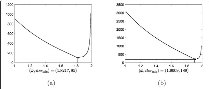
The post-processing algorithm is applied to the linear obstacle problem in -D involv-ingϕ=ϕ. Table  contains efficiency results that compare performances of the PDLP,

the obstacle SOR (without post-process), and the obstacle SOR with the post-process

Table 5 CPU time and iteration comparisons for the suggested post-process, applied to the linear problem withϕ=ϕ2

(ε= 10–7_{) PDL1P Obstacle SOR Obstacle SOR+PP}

Resolution Iter CPU Iter CPU Iter CPU

25×25 814 0.07 56 0.02 92 0.07

50×50 1,486 0.40 108 0.03 147 0.10

100×100 2,092 2.26 213 0.13 299 0.26

200×200 2482 10.47 416 0.84 570 1.34

Table 6 L∞andL2_{error comparisons for the suggested post-process, applied to the linear} problem withϕ=ϕ2

(ε= 10–7_{) PDL1P Obstacle SOR Obstacle SOR+PP}

Resolution L∞error L2_{error L}∞_{error L}2_{error L}∞_{error L}2_error

25×25 1.94·10–2 4.35·10–3 1.94·10–2 4.38·10–3 8.44·10–4 2.80·10–4 50_×50 4.38_·10–3 _8.10·10–4 _4.39·10–3 _8.41·10–4 _2.01·10–4 _6.93·10–5

100×100 1.25·10–3 _2.73·10–4 _1.25·10–3 _2.87·10–4 _5.16·10–5 _1.79·10–5

200×200 5.45·10–4 _7.29·10–5 _5.46·10–4 _7.76·10–5 _1.40·10–5 _4.74·10–6

Figure 11 Plots of the error (uh–u∗) at the 50×50 resolution for the linear obstacle problem with ϕ=ϕ2. (a)by the PDL1P,(b)by the obstacle SOR, and(c)by the obstacle SOR+PP.

(Obstacle SOR+PP) at various resolutions; while Table  presents an accuracy compar-ison for those methods. According to Table , the post-processed solution requires about % more iterations than the non-processed one; the incorporation of the post-process makes the iterative algorithm as twice expensive measured in CPU time as the original iteration. However, one can see from Table  that the post-process makes the error reduced by a factor of ∼. Thus in order to achieve a three-digit accuracy in the maximum-norm, for example, the PDLP requires . seconds and the obstacle SOR completes the task in . seconds; when the obstacle SOR+PP takes only . sec-ond.

Figure  includes plots of the error (uh–u∗) at the × resolution for the linear

obstacle problem withϕ=ϕ, produced by the PDLP, the obstacle SOR, and the obstacle

5.4 Parameter choices

Finally, we present experimental results for parameter choices, when the obstacle SOR is applied for the linear problem withϕ=ϕ. For an effective calibration of the optimal

relaxation parameter as suggested in (.), we first selecth= /. Then by using a

trial-by-error method, we found the calibrated optimal relaxation parameterωh= ., which

results in the following calibrated constant:

c≈.. (.)

Thus it follows from (.) that the calibrated optimal relaxation parameter reads

ωcal,h≈ ⎧ ⎪ ⎪ ⎪ ⎨ ⎪ ⎪ ⎪ ⎩

. whenh= /, . whenh= /, . whenh= /, . whenh= /,

(.)

which is used for the results of the obstacle SOR included in Table .

In order to verify effectiveness of the calibration, we implement a line search algorithm to find a relaxation parameterωthat converges in the smallest number of iterations with ε= –_{, the same tolerance as for the results in Table . Forh= / andh= /, the}

line search algorithm returned the curves as shown in Figure  with

[ω, iter]≈

⎧ ⎪ ⎨ ⎪ ⎩

[., ] whenh= /, [., ] whenh= /, [., ] whenh= /.

(.)

Note that when the calibrated parameters are used, the iteration counts of the obstacle SOR presented in Table  are , , and , respectively, forh= /,h= /, and

h= /. Thus the calibrated optimal parameters in (.) are quite accurate for the op-timal convergence.

6 Conclusions

Although various numerical algorithms have been suggested for solving elliptic obstacle problems effectively, most of the algorithms presented in the literature are yet to be im-proved for both accuracy and efficiency. In this article, the authors have studied obstacle relaxation methods in order to get second-order finite difference (FD) solutions of obsta-cle problems more accurately and more efficiently. The suggested iterative algorithm is based on one of the simplest relaxation methods, the successive over-relaxation (SOR). The iterative algorithm is incorporated with subgrid FD methods to reduce accuracy de-terioration occurring near the free boundary when the mesh grid does not match with the free boundary. For nonlinear obstacle problems, a method of gradient-weighting has been introduced to solve the problem more conveniently and efficiently. The iterative algorithm has been analyzed for convergence for both linear and nonlinear obstacle problems. An effective strategy is also presented to find the optimal relaxation parameter. The resulting obstacle SOR has converged about one order faster than state-of-the-art methods and the subgrid FD methods could reduce the numerical errors by one order of magnitude.

Competing interests

The authors declare that they have no competing interests.

Authors’ contributions

All authors have participated in the research and equally contributed to the writing of this manuscript. All authors read and approved the final manuscript.

Author details

1_{Department of Mathematics, Sogang University, Ricci Building R1416, 35 Baekbeom-ro, Mapo-gu, Seoul, 04107, South} Korea. 2_{Centennial Christian School International, 20 Shin Heung Ro 26-Gil, Yongsan Gu, Seoul, 140-833, South Korea.} 3_{Mississippi State University, Mississippi State, MS 39762-5921, USA.}

Acknowledgements

S. Kim’s work is supported in part by NSF grant DMS-1228337. Tai Wan (the second author) is a high school student who has spent many hours working on mathematical analysis and computational algorithms. S. Kim much appreciates his efforts for the project. Constructive comments by two anonymous reviewers improved the clarity of the paper and are much appreciated.

Received: 5 November 2016 Accepted: 25 January 2017

References

1. Bartels, S: The obstacle problem. In: Numerical Methods for Nonlinear Partial Differential Equations. Springer Series in Computational Mathematics, vol. 47, pp. 127-152. Springer, Berlin (2015)

2. Caffarelli, L: The obstacle problem revisited. J. Fourier Anal. Appl.4(4-5), 383-402 (1998)

3. Cha, Y, Lee, GY, Kim, S: Image zooming by curvature interpolation and iterative refinement. SIAM J. Imaging Sci.7(2), 1284-1308 (2014)

4. Kim, H, Cha, Y, Kim, S: Curvature interpolation method for image zooming. IEEE Trans. Image Process.20(7), 1895-1903 (2011)

5. Kim, H, Willers, J, Kim, S: Digital elevation modeling via curvature interpolation for LiDAR data. Electron. J. Differ. Equ.

23, 47-57 (2016)

6. Petrosyan, A, Shahgholian, H, Uraltseva, N: Regularity of Free Boundaries in Obstacle-Type Problems. Graduate Studies in Mathematics. Am. Math. Soc., Providence (2012)

7. Rodrigues, JF: Obstacle Problems in Mathematical Physics. Notas de Matematica, vol. 114. Elsevier Science, Amsterdam (1987)

8. Arakelyan, A, Barkhudaryan, R, Poghosyan, M: Numerical solution of the two-phase obstacle problem by finite difference method. Armen. J. Math.7(2), 164-182 (2015)

9. Brugnano, L, Casulli, V: Iterative solution of piecewise linear systems. SIAM J. Sci. Comput.30(1), 463-472 (2008) 10. Brugnano, L, Sestini, A: Iterative solution of piecewise linear systems for the numerical solution of obstacle problems.

arXiv:0912.3222 (2009)

11. Hoppe, RHW, Kornhuber, R: Adaptive multilevel methods for obstacle problems. SIAM J. Numer. Anal.31(2), 301-323 (1994)

12. Gräser, C, Kornhuber, R: Multigrid methods for obstacle problems. J. Comput. Math.27(1), 1-44 (2009) 13. Tran, G, Schaeffer, H, Feldman, WM, Osher, SJ: AnL1_{penalty method for general obstacle problems. SIAM J. Appl.}

Math.75(4), 1424-1444 (2015)

15. Chambolle, A, Pock, T: A first-order primal-dual algorithm for convex problems with applications to imaging. J. Math. Imaging Vis.40(1), 120-145 (2011)

16. Esser, E, Zhang, X, Chan, TF: A general framework for a class of first order primal-dual algorithms for convex optimization in imaging science. SIAM J. Imaging Sci.3(4), 1015-1046 (2010)

17. Sochen, N, Kimmel, R, Malladi, R: A general framework for low level vision. IEEE Trans. Image Process.7(3), 310-318 (1998)

18. Zhu, M, Chan, T: An efficient primal-dual hybrid gradient algorithm for total variation image restoration. CAM Report 08-34, Department of Mathematics, Computational Applied Mathematics, University of California, Los Angeles, CA (2008)

19. Zhu, M, Wright, SJ, Chan, TF: Duality-based algorithms for total-variation-regularized image restoration. Comput. Optim. Appl.47(3), 377-400 (2010)

20. Lions, PL, Mercier, B: Splitting algorithms for the sum of two nonlinear operators. SIAM J. Numer. Anal.16(6), 964-979 (1979)

21. Majava, K, Tai, XC: A level set method for solving free boundary problems associated with obstacles. Int. J. Numer. Anal. Model.1(2), 157-171 (2004)

22. Wang, F, Cheng, X: An algorithm for solving the double obstacle problems. Appl. Math. Comput.201(1-2), 221-228 (2008)