Nonclassical excitation and quantum interference in a three level atom

(1)

Nonclassical Excitation and Quantum Interference

in a Three Level Atom

Thesis by

Nikos Photakis Georgiades

In Partial Fulfillment of the Requirements for the Degree of

Doctor of Philosophy

California Institute of Technology Pasadena, California

1998

(2)

©

1998

(3)

Acknowledgements

A person hardly ever walks the path of learning alone. To complete my Ph.D. in Physics was a dream and a goal inspired more than fifteen years ago while I was still at high school learning my first physics from an excellent teacher, Ms. Georgia Stylianou, who not only encouraged but also promoted my interests in science. Alongside with my high school teacher, at the dawn of my scientific awakening, the fascinating TV series Cosmos by Prof. Carl Sagan triggered my curiosity and brought my young and unshaped mind in front of the amazing wonders of the universe. Since then many wonderful teachers have taken me under their wings and taught me science. Among the most prominent of them were some of my college professors at the University of Pennsylvania to whom I would like to give special thanks: Prof. Rex Rivolo, Prof. Borris Lerner, Prof. Paul Soven and Prof. Fay Ajzenberg-Selove. My undergraduate research advisor Prof. Argun G. Yodh needs special mention since he was the one who introduced me to the world of scientific research and guided my first steps through a "real" scientific project. However, I would not have been able to write this thesis if it were not for one more teacher of mine, a professor at Caltech, with whom I spent the last six years developing my scientific skill and personality. This professor is, of course, none other than my research advisor Prof. H. Jeff Kimble. From Professor Kimble not only did I learn physics, but I also learned about scientific integrity, about being a hard and fair judge, about being competitive and the meaning of being a "good scientist." Prof. Kimble has been to me a teacher, a raw model, a guide and a friend. For all that he has offered me, I would like to express to him my gratitude, appreciation and very special thanks. In addition to my advisor, of extreme importance to my graduate school career was our entire research group that often felt as an extended family within which I could seek help, recognition and comfort. My "lab mentor"

(4)

(5)

Abstract

(6)

scheme to other energy triplets and atoms, leads to the discovery that ranges up to

100' s of TH z can be bridged in a single mixing step. Motivated by these results, a master equation model has been developed for the system and its properties have

(7)

I

BASIC EXPERIMENTAL CONCEPTS

2 Magneto-Optical Trap

2.1 Geometry . . .

17

18

19

20

21

(8)

2.2 Trapping Beams . 2.3 Magnetic Fields

2.4 Alignment

2.4.1 MOT Alignment

2.4.2 Excitation Fields 2.4.3 Imaging

2.5 Summary

3 High Precision Spectroscopy of the 6D5;2 State in Cs

3.1 Two-Photon Spectroscopy in a MOT vs. in a Vapor Cell 3.2 Experimental Setup . . . . . . . . . . .

3.2.1 Locking and Scanning (Block I)

3.2.2 Detection and Data Acquisition (Block IV) . 3.3 Theory of hf Structure for the 6D5;2 State

3.4 Results . . . .

3.5

3.4.1 The a and b Coefficients 3.4.2 Linewidths . . . . . . . .

3.4.3 AC Stark Shift of the Ground State . 3.4.4 "Cross-Talk" between hf States Summary . . . .

4 Optical Parametric Oscillator

4.1 OPO Configuration . . .

4.1. l Cavity Elements 4.1.2 Beam Paths . . 4.1.3 OPO Locking . 4.1.4 Triangular Cavity . 4.2 Degenerate Operation . .

4.2.1 Phase-Sensitive Gain 4.2.2 Squeezing Spectra . .

4.2.3 Summary of the DOPO Results

(9)

4.3 Non-Degenerate Operation

4.3.1 Operation . . 4.3.2 Performance .

4.4 Summary . . . . . .

II

SQUEEZED LIGHT AND ATOMS

5 Two-Photon Excitation Rate with Nonclassical Fields: Experiment

5.1

5.2

5.3

Theory.

5.1.1 "Simple" Theory

5.1.2 "Full" Theory . .

5.1.3 Classical versus Nonclassical Effects .

Experiment

5.2.1 Setup

5.2.2 ON/OFF Protocol

5.2.3 Background

5.2.4 Data .

5.2.5 Control Experiment .

Summary

Theory and

6 Two-Photon Excitation Rate with Nonclassical Fields: Analysis,

65 66 68 72

74

75 76 76 79 80 83 83 84 86 87 90 92

Statistics and Results 94

6.1 Statistical Analysis Part I: Functional Form of R2 vs.

Ri

94

6.1.1 Fitting Procedure . 94

6.1.2 The S statistic 98

6.1.3 The C statistic 99

6.1.4 fQ VS fQ+L 100

6.2 Statistical Analysis Part II: The G factor 101

(10)

6.4 Combining all Data .

6.5 Summary . . . .

III

QUANTUM

INTERFERENCE

109

113

114

7 Multiple-Field, Two-Photon Excitation and Quantum Interference 115

7.1 The 3-level Atom and Excitation Scheme

7.2 Perturbative Analysis . .

7.2.1 Equation of Motion .

7.2.2 Solution for p33 and QI .

7.3 "Full" Theory . ..

7.3.l Hamiltonian Formalism .

7.3.2 Equation of Motion .

7.3.3 Solution

7.4 QuinC

7.5 Experiment

7.6 Multiphoton Excitations

7.7 Internal State Correlations

7.8 Summary

8 Ultrafast Homodyne Detection

8.1 Theory.

8.1.1 Excitation Field .

8.1.2 Hamiltonian Formulation and Master Equation

8.1.3 Equations of Motion

8.1.4 Solution for the Atomic Populations .

8.2 Experiment

8.3 Summary

9 Atoms as Ultrafast Nonlinear Mixers

9.1 Characterization of Atomic Nonlinear Mixers .

(11)

9.1.1 ANM Frequency Response with Fixed Excitation Power . 159 9.1.2 ANM Frequency Response with Variable Excitation Power 162

9.2 Database of Atomic Nonlinear Mixers . 9.3 Frequency Metrology . .

9.4 Optical Communication 9.5 Summary

10 Epilogue

A OPO Gain for the Single and Double-Sided Cavity

A.1 Degenerate OPO (DOPO) . . . A.1.1 Probe Injected Through M1 A.1.2 Probe Injected Through Mout A.2 Non-Degenerate OPO (NDOPO)

A.2.1 Probe Injected Through M1

A.2.2 Probe Injected Through Mout

A.3 Summary . . . .

163 165 168 169 170 173 173 176 176 177 180 180 181

B Nonclassical Two-Photon Experiment: Data Plots, Fits and Fit Pa

-rameters 182

B.1 Exp. 11-17-94 (Nonclassical Excitation) . 183 B.2 Exp. 11-29-94 (Nonclassical Excitation) . 184 B.3 Exp. 12-06-94 (Nonclassical Excitation) . 185 B.4 Exp. 12-20-94a (Nonclassical Excitation) 186

B.5 Exp. 12-20-94b (Nonclassical Excitation) 187

B.6 Exp. 12-22-94 (Coherent Excitation) 188

B.7 Exp. 01-12-95 (Coherent Excitation) 189 C Results from Numerical Integration of the Master Equation for the

N onclassical Two-Photon Excitation Experiment

C.1 Master Equation . . .

C.2 Parameters and Notation .

(12)

C.3 Results . . .

C.4 "Knee Position"

193

195

D Effect of Detunings on the "Knee" Position in the N onclassical

Two-Photon Excitation Experiment 199

(13)

List of Figures

1.1 A three-level system is realized by considering an "isolated' energy

submanifold of an alkali atom. . . . . . . . . . . . . . . . . . . . . . . 2

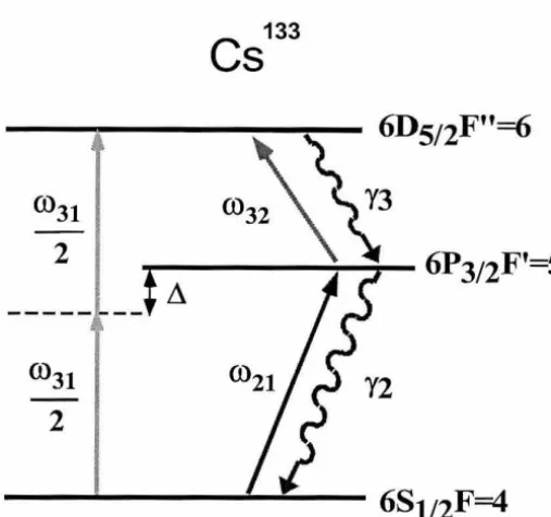
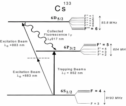
1.2 The three-level energy submanifold in atomic Cesium which was used

in our experiments. . . . . . . . . . . . . . . . . . . . . . 5

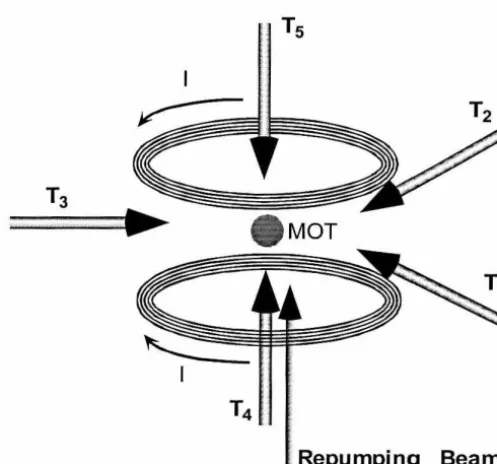
1.3 MOT setup: five trapping beams, T1, ...

,

Ts

,

and one repumping beam are responsible for cooling the atoms. A pair of coils with antiparallel

currents,

I

,

produce a magnetic field gradient which in concert with

the light force confine the atoms in a localized region in space.

1.4 NDOPO setup for producing nonclassical light.

1.5 Interaction of atoms with classical and squeezed vacuum, shown as

circles and ellipses, respectively. . . . . . . . . . . . . . . .

7

g

11

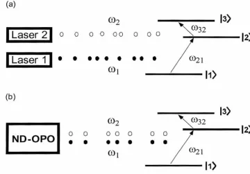
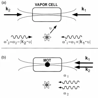
1.6 (a) Classical and (b) quantum excitation of a two-photon transition. 12

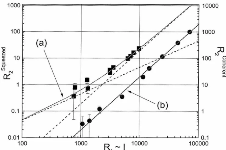
1.7 Experimental observation of two-photon excitation with (a) quantum

correlated and (b) classical fields. The units of the counting rates,

Rf queezed and Rf oherent, are detected photons/ sec. The solid lines are

fits to the data of the form of Eqs.(1.3) and (1.4), while the dotted lines

are the linear and quadratic components plotted separately for the fit

to the non-classical data. The x - axis is a measure of the intensity in arbitrary units. . . . . . . . . . . . . . . . . . . . . . . . . . . 15

1.8 Excitation of a two-photon transition by three phase-coherent lasers

leads to quantum interference. . . . . . 16

2.1 The xy - plane geometry of the MOT. 22 2.2 Imaging of the trap. A one-to-one telescope collects light from the

(14)

3.1 Doppler free spectroscopy: (a) using counter propagating beams in a

vapor cell, (b) using co-propagating beams in a MOT. . . . . . . 31

3.2 Focusing geometry of the excitation beam. Notice that the volume of

excited atoms that is imaged may be smaller than the diameter of the

trap . . . .

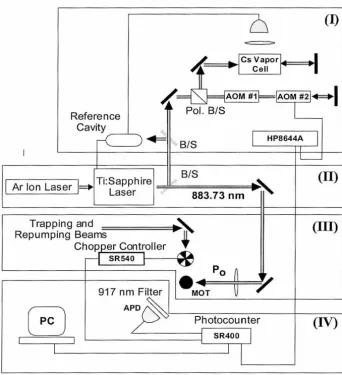
3.3 Experimental setup.

3.4 Hyperfine structure of atomic C s133.

3.5 Hyperfine spectrum of the 6D5;2 state in C s133.

3.6 Linewidth of the hf components of the 6D5; 2 state as a function of

power of the excitation beam. .

3.7 Two-photon excitation spectra, which show Stark shifts and power

broadening due to perturbation of the ground state by the trapping

beams. a) Trapping beams are OFF, b) Trapping beams ON, total

power PJb) ,...., 3.1 mW, c) Trapping beams ON, total power PJcl ,...., 10.4

mW. The power of the 884 nm, two-photon excitation beam, is 3.3

mW in each case. . . . . . . . . . . . . . . . . . . . .

3.8 Cross-talk m as a function of the probe frequency

w (w

=

0 is the

resonant frequency with the F"

=

6 state) . . . .

4.1 A basic OPO consists of a non-linear crystal,

x<

2_l_insid_{e a}_n _optical

cavity. The OPO is pumped by a laser at frequency wp and generates

a signal and idler output at frequencies W8 and wi, respectively.

4.2 OPO geometry . . . .

4.3 Experimental setup to generate squeezed light.

32

35

41

42

43

45

47

49

50

53

4.4 Phase-sensitive gain of a coherent beam transmited through the DOPO. 55

4.5 OPO gain G+ vs. the dimensionless pumping parameter x2

. The

solid line is the theoretical prediction (G+

=

(1 -

x)

-

2) with no free

(15)

4.6 OPO gain G_ vs. the dimensionless pumping parameter x2

. The

solid line is the theoretical prediction (G_

=

(1

+

x)-

2) with no free

parameters. . . . . . . . . . . . . . . . . . . . . . . . . . . 57

4.7 The product G+G- versus the dimensionless pumping parameter x2.

The solid line is the theoretical prediction G+G- = (1 - x2

) -2. . . 58

4.8 OPO amplification gain G + versus deamplification G _ for all

measure-ments. The solid line is the theoretical prediction G + = G _ ( 2~ - 1 )-2. 59

4.9 Balanced homodyne detector. . .

61

4.10 A typical spectrum of squeezing. . 62

4.11 The squeezed (.6.X_ = 1 + S_) versus the antisqueezed ('6.X+ = 1

+

S+) quadratures of the OPO output. The solid line is the minimum

uncertainty relation '6.X+.6.X_ = 1. .

4.12 The squeezed (.6.X_ =

l

+S_)

versus the antisqueezed ('6.X+ =

l+S+

)

quadratures of the OPO output calculated taking into account an extra

efficiency factor (x. The solid line is the minimum uncertainty relation

64

'6.X+.6.X_ = 1. . . . . . . . . . . . . . . . . . . . . . 65

4.13 Schematic representation of double resonance in the NDOPO. The

ver-tical lines denote longitudinal modes of the OPO cavity for the two

wavelengths As (solid lines) and Ai (doted lines), which are separated

by As and ,\, respectively. As the cavity length is changed, the r

eso-nances of the two wavelengths move relative to each other until they

coincide and to produce another double resonance.

4.14 When the OPO cavity is doubly resonant with the injected w852 and

conjugate w 442 - wss2 frequencies, there is amplification of the injected

beam.

4.15 Sequence of measurements to determine the OPO gain: (a) no-gain

measurement of the transmitted power

Vo;

(b) combined power of the

amplified 852 nm and generated 917 nm beams,

1/8

52+917 ; (c) amplified

power of the injected beam at 852 nm alone, V852 ; (d) generated power

of the idler beam at 917 nm alone, \.l~ll7·

67

68

(16)

4.16 Plot of the gain measurements of the idler beam G~~~ 1 versus G~~~ 2,

which were determined by two independent methods. For the data to be consistent, they must fall on the diagonal G~~~ 1 = G~~~ 2. 71

4.17 Idler gain G~~~ versus signal gain G~~~. The solid line is the theoretical prediction for the relation of the two, namely

G~~~

=

G

~~

~

( 1 -

~

)

. 72

5.

1

Two-photon excitation by non-classical fields: a three-level atom

{11

)

, 12) , 13)}

is illuminated by the signal and idler (ws,wi) output beams from an NDOPO, and they are near resonance with the

11 )

--+

12 )

and

12 )

--+

13 )

transitions, respectively (ws c:::: w₁₂and wi c:::: W23). . . . 75

5.2

The output field Eaut of the OPO is related to the input state Ein via

the transformation Eout = µEin

+

ZJ Efn. . . . . . . . . . . . . . . 77

5.3

Quadrature space of the squeezed states of the electromagnetic field. Curve (i) indicates minimum uncertainty states which satisfy ~X-~X+ =

1. Curve (ii) corresponds to thermal states for which ~X- = ~X+

>

1. Curves (iii) and (iv) are for states with ~X+

=

1 and ~X-

=

1, respectively. States in region (a) are forbidden by the uncertainty r e-lation. States in region (b) are quantum squeezed states characterized by the fact that either ~X+

<

1 or ~X-

<

1. States in region (c) are classically squeezed states with both ~X+

2'.:

1 and ~X-

2'.:

1 and also with unequal quadratures ~X- -=/- ~X+. The special state ~X- = ~X+ = 1 corresponds to the electromagnetic vacuum. . . . . 82 5.4 Experimental setup for two-photon excitation with non-classical fields. 83 5.5 a) With the trapping beams turned ON, the rate R1 is proportional to

the intensity of the idler field. b) When the trapping beams are turned OFF, the rate R2 is proportional to the two-photon excitation rate by

the signal and idler beams from the NDOPO. 85 5.6 Gating of the photon counter. Gate A corresponds to the OFF and

(17)

5.7 Setup for generating two coherent beams at 852 nm and 917 nm in resonance with the 6S1;2F

=

4 ~ 6P3;2F'

=

5 and 6P3;2F'

=

5 ~

6D5; 2F" = 6 transitions, respectively.

6.1

R

2 versus

R

1 from the nonclassical two-photon excitation experiment

of 12/20/94-b. The solid line is a quadratic plus linear fit

(f

Q+L) and 92

the dotted line is a quadratic fit (JQ)· . . . . . . . . . . . . . . . . 102 6.2

R

2 versus

R

1 from the two-photon classical excitation experiment of

12/22/94. The solid line is a quadratic fit

(f

Q)

to the data. . . . . 103 6.3 One photon counting rate R1 versus the OPO gain G852 from the data

of 11/29 /94. The solid line is a fit of the form R1 = a1 ( ~ - 1). . 104 6.4 Two-photon counting rate R2 versus the OPO gain G852 from the data

of 11/29 /94. The solid line is a fit of the form R2 = a2 ( ~ - 1)

+

a3 (

~

- 1)

2

. The dasshed lines shows the quadratic fit of the form

R

2

=a~(~

- 1)

2

. . . 105 6.5 Gain at the knee position G~nee for the non-classical excitation

experi-ments. The solid line at G = 1.33 is the prediction from the full theory

and is approximately the sames as the value predicted from the theory of Ficek and Drummond. The solid line at G

=

1.41 is the average of the experimental values and the two dotted lines symmetrically around it are the la error bars. . . . . . . . . . . . . . . . . . . . 108

6.6 Excited state population p33 due to nonclassical two-photon excitation as a function of OPO output intensity expressed in terms of the intra

-cavity photon number for the idler field, n917. The solid line is the full theory and the dotted lines are the linear and quadratic asymptotes

to the theory. The data points are the normalized data from the five

experiments. . . . . . . . . . . . . . . . . . . . . . . . . . llO 6.7 Residuals of the normalized data (a) relative to the quadratic and (b)

(18)

7.1 The two-photon transition 11) -+ 13) is excited by three fields via two

alternative excitation pathways, which lead to QI. . . . . . . . 116

7.2 Quantum Interference Calculator (QuinC) is available on the

WWW

at http://www.cco.caltech.edur qoptics/QIHome/QuinC/QuinC.html 131

7.3 Setup for the QI experiment. . . . . . . . . . . . . . . . . . 133

7.4 Fluorescence from the 6D5;2F"

=

6 -+ 6P3; 2F'

=

5 transition as a

function of time for excitation of the atoms in the MOT by a

combina-tion of three coherent beams with corresponding wavelengths 852 nm,

917 nm and 884 nm. The phase of the 884 beam is modulated with a

PZT at a frequency ~ ~ 11 Hz. . . . . . . . . . . . . . . . . . . 134

7.5 Multiphoton excitation with multiple lasers {w1, w2, ... ,wk}· Several

excitation paths

{X

1,

X

2, ....

Xm}

contribute to the overall excited state

population Pnn, resulting in QI. . . . . . . . . . . . . . . . . . 136

7.6 Atomic state populations p 11, P22 and p₃₃ as functions of the phase

e

'

calculated from the full theory model using a =

j!r,'

81 = -

~

'

f: - 10 f: - 61 +62 d " - " -

Q

-

2

u2 - - v'45, uo - ₂ an ~'I - ~ '2 - o - . . . .

8.1 Two-photon excitation by a combination of a coherent RO field with

frequency w0 , in resonance with the two-photon 11) -+ 13) transition,

and the signal and idler outputs of an NDOPO at frequencies W8 and

wi in resonance with the dipole 11) -+ 12) and 12) -+ 13) transitions,

respectively. . . . . . . . . . . . . . . . . . . .

8.2 a) Homodyne detection of squeezing. b) Detection of nonclassical co

r-138

141

relations with QI where an atom is utilized as a nonlinear mixer. 142

8.3 Experimental setup for observation of QI with squeezed light.

8.4 Power spectrum R (!) of the photocounting time series fp. a) Control

spectrum with the squeezing turned off for which no modulation at

either Wm or 2wm is observed; b) spectrum with the squeezing on for

which a peak at frequency 2wm appears.

153

(19)

9.1 A three level atom acting as a nonlinear mixer. Three input fields at

frequencies w1 , w2 and w3 are "mixed" to result in a "demodulated"

output signal. . . . . . . . . . . . . . . . . . .

9.2 Frequency response of pin (a), (b) and (c) and Vin (d), (e) and (f) as

functions of the detuning 8. Solid lines are for 81 = 8, 82 = 0, 80 = O;

dotted lines are for 81 = 0, 62 = 6 , 60 = O; dashed lines are for 81 = 0,

62 = 0, 80 = 6. The value of a=

j!f;

is for (a) and (d) a=

[Fa,

for

(b) and (e) a =

ji

and for (c) and (f) a =

j¥.

Note that 8 is in 158

units of / =

fi?i3.

.

. .

.

. .

. . .

.

. . . . .

.

160

9.3 Full width at half maximum

6..

~~HM>

i = 0, 1, 2 for the visibility V as

a function of a=

/!I;

·

Note that

6..~~HM

is in units of/ =

fi?i3

.

162 9.4 From the three possible two-photon excitation schemes, 3, V and A,

only the first one is considered here. The other two also exhibit QI and

could be also used as nonlinear mixers. . . . . . . . . . . . . 164

9.5 ANM characteristics for the sideband-to-carrier separation 6..f versus

the carrier wavelength Ac for the database of 6900 transitions in the

alkali elements. The circled point corresponds to the experimental

demonstration with Ac~ 884 nm and 6..f ~ 12.5 THz. . . . . . . 166

9.6 By frequency sum and difference generation and harmonic conversion

( Wi

±

Wj), an initial Set of reference frequencies fl0 together with the target frequency Wt results after k stages of nonlinear transformations

into a new set of frequencies

nk

.

From

nk

the three "best" frequencies

{ Wa, wb,

w

e

}

for the particular application are chosen.

A. l DOPO configuration. .

A.2 NDOPO configuration.

B.l a) R2 vs. R1 data from the 11-17-94 experiment. The solid line is the

best linear plus quadratic fit and the dashed line the best quadratic

fit. b) Quadratic plus linear residual, define in Eq. (B.l) c) Quadratic

residual, defined in Eq. (B.2)

167

174

178

(20)

B.2 a) R2 vs. R1 data from the 11-29-94 experiment. The solid line is the

fit. b) Quadratic plus linear residual, define in Eq. (B.l) c) Quadratic residual, defined in Eq. (B.2) . . . . . . . . . . . . . 184

B.3 a) R₂vs. R₁data from the 12-06-94 experiment. The solid line is the best linear plus quadratic fit and the dashed line the best quadratic

fit. b) Quadratic plus linear residual, define in Eq. (B.l) c) Quadratic

residual, defined in Eq. (B.2) . . . . . . . . . . . . . . . . 185 B.4 a) R2 vs. R1 data from the 12-20-94a experiment. The solid line is the

fit. b) Quadratic plus linear residual, define in Eq. (B.l) c) Quadratic residual, defined in Eq. (B.2) . . . . . . . . . . . . . . . 186 B.5 a) R2 vs. R1 data from the 12-20-94b experiment. The solid line is the

fit. b) Quadratic plus linear residual, define in Eq. (B.1) c) Quadratic residual, defined in Eq. (B.2) . . . . . . . . . . . . . . . . . . . 187 B.6 a) R2 vs. R1 data from the 12-22-94 experiment. The solid line is the

best linear plus quadratic fit and the dashed line the best quadratic fit. b) Quadratic plus linear residual, define in Eq. (B.1) c) Quadratic residual, defined in Eq. (B.2) . . . . . . . . . . . . . . . . . . 188 B.7 a) R2 vs. R1 data from the 01-12-95 experiment. The solid line is the

best linear plus quadratic fit and the dashed line the best quadratic fit. b) Quadratic plus linear residual, define in Eq. (B.1) c) Quadratic

(21)

C.l a) Circles: Excited state population p₃₃as a function of the intracavity

photon number of the idler mode nb from numerical integration of the

master equation by A. S. Parkins. b) Solid line: "Phenomenological"

fit to the numerical data of the form

p~;)

=

ec:nb

+

f3n~

( 1 -

1e

-

!!:f

).

c)

Dashed line: Best linear plus quadratic fit to the numerical data of the form p~;) = ec:'nb

+

f3'n~. d) Insert: Ratio of the two fits shown in (b)

C.2

(1) and (c), ~ -Paa

Log-log slope ddllogpaa as a function of the idler intracavity photon-ognb

number nb. a) Slope of p~;) (solid line); b) slope of p~;) (dashed line); c) slope of

pf

p

(

TJ

«

1) (dotted line). . . . . . . . . . . . . . . .

194

(22)

List of Tables

4.1 Raw data of P, G+ and G_ for the experiments of 2/11/94, 4/2/94,

5/2/94 and 8/4/94. Note that Pis in mW. . . . . . . . . . . . . 60

4.2 Size of the squeezing R_ and antisqueezing R+ relative to the shot

noise in linear units. Corrections for the finite level of the shot noise

have been included. Pis the pump power in mW. 63 4.3 Gain measurements for the NDOPO. . . . . 70

5.1 Excitation with non-classical fields, data from experiment 11/17 /94. 89 5.2 Excitation with non-classical fields, data from experiment 11/29/94. 90

5.3 Excitation with non-classical fields, data from experiment 12/06/94. 91

5.4 Excitation with non-classical fields, data from experiment 12/20/94-a. 91

5.5 Excitation with non-classical fields, data from experiment 12/20/94-b. 92

5.6 Excitation with coherent fields, data from experiments on 12/22/94 and 1/12/95. . . . . . . . . . . . . . . . . . . . . . . . . . 93

6.1 Significant levels S and

xC

2_{l values for fits to the test functions. The}

number of free parameters n - din the experiments of {11/17 /94, ... ,

1/12/95} are for fQ equal to {18, 7, 12, 6, 11, 8, 9} and for fQ+c, fp and fQ+L equal to {17, 6, 11, 5, 10, 7, 8}. . . . . . . . . . . . . . . . . . 97 6.2 Fit parameters and OPO gain at the lmee position, G~nee, for the

non-classical excitation experiments. . . . . . . . . . . . . . . . . . . . 107

C .1 Data from numerical integration of the master equation appropriate for

the nonclassical excitation experiment of Ch. 4 and 5. (From private

communication with A. S. Parkins, Feb. 1995). . . . . . . . . . . 193

D.l "Knee" position and detunings: data from numerical integration of the

(23)

Chapter

1 Introduction

It may be argued that an atom, especially an alkali with a single electron in its outer

shell, is a very simple physical system. In addition, if one considers only an isolated sub-manifold of few (three in our case) of its energy levels, as in Fig. 1.1, then the dynamics of this atom under the influence of electromagnetic (EM) fields should

be readily understood. Yet, such a simple system has given us enough material to investigate, keeping us occupied for the last six years. In fact, the simplicity of the

three-level system of Fig. 1.1 has been the ideal test bench for the investigation of

otherwise very complicated phenomena. During this time and with the aid of such an

atom, some very fundamental concepts and principles in the field of Quantum Optics

and Atomic and Molecular Physics have been uncovered. The journey of exploration

through this very simple three-level atomic system and the discoveries made along

the way are the subject of my Thesis.

More specifically, using a three-level atom, a variety of new phenomena associated

with the interaction of atoms with various states of the EM field have been

stud-ied. As part of the work, experimental techniques have been developed, nonclassical phenomena have been observed, the system has been studied theoretically and the

acquired lmowledge was extended to practical applications with implications in a

va-riety of fields. The emphasis of the work was divided among two principle subjects:

the investigation of quantum effects associated with the interaction of atoms with

quantum states of the EM field and the quantum features of the interaction of the

atoms with multiple single-mode coherent states of the EM field. A combination of

these two subjects sparked further developments and, as a result, observations have been made of otherwise out of reach nonclassical correlation of fields separated in

(24)

Decoupled

Higher-energy _ _ _ _ _ levels

Full shell Lower-energy levels

.

-Three level

energy sub manifold

.---'

· 13)

~iiiliiiiii-

12)

Unoccupied

Excited states

Ground state occupied by a sing le electron

Figure 1.1: A three-level system is realized by considering an "isolated' energy s ub-manifold of an alkali atom.

The intent is to cover in this Thesis the basic milestones and explain the physical principles of this work. The journey takes us from basic understanding of a three-level

atom to notions such as nonclassical two-photon excitation, quantum interference in

multiphoton excitation and the use of atoms as ultra-fast non-linear mixers. These subjects will all be explained in due time in the subsequent chapters, but before

getting into the details, in the remainder of this chapter a brief overview of the things to come will be outlined.

1.1 The Three

"Eras"

of

my

Research

Reflecting back on the work of the last six years, I see that my Thesis is naturally

divided into three "eras" which I will conveniently use as break points in the discussion

of our research. The first "era" I call "Basic Experimental Concepts." During this time some of the fundamental experimental techniques and methods needed for the subsequent work were developed. At this preliminary stage a magneto-optical trap

(25)

sample for the subsequent experiments. Following this, the capability to perform

high-resolution spectroscopy on the atoms in the MOT was developed and measurements

of the previously unresolved internal structure of the third excited state of the atom

were performed. Finally, a unique facility capable of producing frequency tunable

squeezing was modified to match the needs of the research program that followed.

During this era the foundations of my experimental skills were put into place.

The next "era" was the time when one of the most challenging tasks in Quantum

Optics, namely the observation of nonclassical effects associated with the interaction

of squeezed light with atoms, was undertaken. This em I call "Squeezed Light and

Atoms." During this time pioneering experiments were performed and for the first

time complemented with observations, theoretical predictions that existed for more

than a decade. [1] Here an example of nonclassical behavior of atoms interacting with

squeezed light as manifested in two-photon excitation by correlated pairs of photons

was demonstrated. In particular, the excitation rate as a function of intensity was

measured to deviate from the classical quadratic law and was observed to

asymp-totically approach a linear dependance in accordance with theory. Until today, the

work of this era has been the only successful attempt, and with the exception of an

alternative, relatively unsuccessful approach also implemented by us, [2] it remains

the only experiment on the subject.

Finally we come to the third "era," the era of "Quantum Interference." This

has been the most productive era of my graduate career, where as a well "seasoned"

student I have produced the bulk of my work. During this time, by modifying the

previous experiment, a two-photon transition was excited by using multiple photons.

As a result there were more than one possible excitation pathway, which lead to

Quantum Interference (QI). Not long after the initial observations, it was realized

that this could have profound implications in several fields. The key idea is that

atoms act as ultrafast nonlinear mixers due to QI. First by applying these findings to

frequency metrology, we proposed novel techniques for bridging large frequency gaps

in single steps. Then we applied our results to optical communications and obtained

(26)

homodyne scheme and presented a proof-of-principle experiment in support of our claim. Finally, in order to lay some solid ground for future work on the subject, we have theoretically analyzed the details of our system by solving the master equation that produced models valid in a large range of parameters.

With this prelude in mind we now turn to the more technical discussion. The next section is devoted to introducing the atomic system used throughout our experiments, while the following three sections are an overview of the science of each of the ems mentioned above. Here, the goal is to relate to the reader the main concepts and key ideas that will appear in the rest of the Thesis and summarize the content of the various chapters. The interested reader may then refer for more details to the subsequent chapters.

1.2 Three-Level Energy Submanifold in

Cs

133

The particular atom that was used throughout our experiments is atomic Cesiurn-133. The relevant transitions that comprise the three-level energy submanifold of Fig. 1.1 are the 6S1;2F

=

4, 6P3;2F'

=

5 and 6D5;2F"

=

6 states, as shown in Fig. 1.2. To

familiarize further the reader with the atomic system of Fig. 1.2, it is worthwhile to introduce at this point the notation and parameters which will be used repeatedly throughout the rest of this Thesis. First, the simplifying notation {11), 12), 13)} is employed to denote the energy levels {6S1;2F

=

4, 6P3;2F'

= 5,

6D5;2F"

=

6}. Then

the eigenfrequencies of the system are defined to be

(1.1)

where Ei is the energy of each state. The eigenfrequencies for the atom in Fig. 1.2 have corresponding wavelengths equal to >-21 '.::::'. 852 nm , A32 '.::::'. 917 nm and _A31'.::::'. 442 nm.

The FWHM atomic linewidths are 'Y2 '.::::'. 5 MHz and 'Y3 '.::::'. 3 MHz and correspond

(27)

important parameter of the system is 6 , which is defined to be

I

W311

I

W31

I

6 - W21 -

2 =

W32 -

2

·

(1.2)

Stated differently, 6 is a measure of the degree of non-degeneracy in the system which

for our case is equal to 6 c:= 25 TH z.

ffi31

2 ....

----""""!""" ... -

6P312F' 5

[image:27.562.165.419.189.427.2]

---

_

__ ; d

Figure 1.2: The three-level energy submanifold in atomic Cesium which was used in

our experiments.

1.3 Ba

s

ic Exp

e

rimental Conc

e

pts

In the first part of the Thesis the basic lab set-up that was used throughout the exper

-iments will be described. This set-up consists of two main components: a frequency

tunable source of squeezed light [3, 4] that generates nonclassical states of the EM

field and a magneto-optical trap (MOT) [5,

6 ]

that provides a Doppler-free atomic

(28)

1.3.1 Magneto-Optical Trap

Starting from the first part of the experimental set-up, the magneto-optical trap (MOT) shown schematically in Fig. 1.3 is formed by a combination of optical and magnetic fields. In particular, five laser beams (two with opposite directions along the

z-axis, and three in the perpendicular plane, spaced by 120° from each other) together with a repumping beam, are responsible for cooling the atoms down to the Doppler limit of 120 µK. In addition, a pair of coils with anti-parallel currents produces a magnetic field gradient, which in concert with light forces produces a potential well in which the atoms are confined. Although this is a well established technique for

cooling and trapping, [5, 6] some of the discussion will nevertheless be devoted in the particular realization in our own experiments in order to document the parameters

and characteristics of the apparatus. To give a general idea of the trap that we had in our disposal, it is worth noting at this point that the physical size of the MOT was of the order of 0.1 - 0.3 mm in diameter, it had a temperature close to the Doppler cooling limit of about 120 µK, its density was estimated to be of the order

of 109 _atoms/_cm3 _and_{hence the}_number_{of atoms in}_{the MOT was of the order of}

500 - 15, 000.

1.3.2 High Precision

Spectroscopy of the

6D

5;2

State

in

Cs

133

Continuing the discussion of the preliminary phase of our research, I will then describe

a classical spectroscopy experiment which was performed in order to study the 6D5;₂

state of Cs.[7] This exercise was a very crucial initial step in our work for a couple of reasons. First, in order to realize an isolated three-level energy submanifold, it is important to know the internal (hyperfine) structure of the states involved in the transitions. However, as it turned out, the 6D5; 2 level had not been carefully studied in the past, and the only available reference [9] until then quoted an accuracy for the measurements of only 30%. In addition, for the experiments that followed it was

(29)

9 MOT

Repumping Beam

Figure 1.3: MOT setup: five trapping beams, T1 , ... , T5 , and one repumping beam

are responsible for cooling the atoms. A pair of coils with antiparallel currents, I, produce a magnetic field gradient which in concert with the light force confine the

atoms in a localized region in space.

Turning now to the actual spectroscopy experiment, it is noted that it was per

-formed by exciting the two-photon transition 6S₁;₂F = 4 - 7 6D₅;₂F" by a tunable

Ti:Sapphire laser and then observing the emitted fluorescence from the cascade decay

back to the ground state. In particular, monitoring of the excited state population was achieved by observing the fluorescence emitted from the 6D_{5; 2}F" - 7 6P₃;₂F' = 5

transition. The main outcome of these measurements was the determination of the

hyperfine structure (hfs) of the 6D5;2 level as characterized in first order by the ma g-netic dipole a and in second order by the electric quadruple b coefficients. These

coefficients were measured to be a= - 4.69

±

0.04 MHz and b = 0.18

±

0.73 MHz.

[image:29.562.151.400.69.301.2]

(30)

This was solved by implementing a chopping cycle (at 4 KHz) for the trapping beams and performing the measurements only during the OFF part of the cycle. However, even the ON part of the cycle was interesting and by comparing spectra obtained during the ON and OFF parts of the cycle, useful information about the magnitude of the Stark shifts and power broadening have been extracted.

A second problem that needed special attention was the signal-to-noise (S/N) ratio of the measurements. First an efficient technique for the observation of the fluorescence from the 6D5;2F" ---+ 6P3;2F' = 5 transition had to be devised and

then the background light (mostly from scattering from the trapping beams which even during the OFF part of the cycle was enough to produce noticeable signals)

had to be dealt with. In addition, during the ON part of the cycle the detector was oversaturating and was not recovering fast enough for the measurements to be made accurately during the OFF part of the cycle. However, by realizing that the wavelength of the trapping beams is 852 nm, while that of the 6D5;2F" ---+ 6P₃;₂F' = 5 transition was close to 917 nm and by using an interference (notch) filter centered at 917 nm, good isolation was provided that helped to overcome these difficulties by eliminating the background to acceptable levels and avoiding detector saturation

from 852 nm light.

1.3.3 Optical Parametric Oscillator

The last chapter of Part I refers to the subthreshold optical parametric oscillator ( OPO) which was the source of radiation for the experiments that followed. The operation of the OPO in two modes, the degenerate (DOPO) and non-degenerate (NDOPO), will be discussed. The setup, particularly of the NDOPO which is relevant for the experiments, consists of a very complex set of optical elements, alignment procedures, optimization techniques and electronic feedback loops (see Fig.1.4), all

(31)

there exists a lot of theoretical [12, 13] as well as experimental [3, 4] work on the subject and most of the setup was already in place. Hence, the emphasis here will be on the operation of the OPO and measurements that were taken to characterize its properties. In addition the modifications that have been introduced and operating

details will be outlined.

Ti:Sapphire Laser

Feedback

·-

-

.

- -

--

-BS

l

883 nm

...

Doubling _Cavity

ND-OPO

442 nm

-.

_{_.}

Signal

___

_-

_{- -}

,

__

- -

852 nm - - - -

_-

_ _

_-

-

-Idler, 917 nm

Figure 1.4: NDOPO setup for producing nonclassical light.

Perhaps the most important modification in the system of Ref. [3, 4] is the fact

that in this case the OPO was operating in a non-degenerate mode producing signal and idler beams that were separated in frequency by 25 TH z and had respective

wavelengths of 852 and 917 nm. Not only was it a challenge to operate the OPO

cavity in this large non-degenerate mode (which effectively means that the cavity had to be in double resonance with the signal and idler frequencies), but also the signal and idler frequencies had to be resonant with the 11) --> 12) and 12) --> 13)

transitions, respectively, for the nonclassical spectroscopy experiments to be feasible. These challenges are unique tasks that had to be accomplished for the first time.

(32)

with theoretical predictions will be discussed. In particular, measurements of the spectrum of squeezing for the degenerate OPO that verify the uncertainty relation for conjugate quadratures of the electromagnetic field will be presented, and data on phase-sensitive gain will be shown and compared to phase-sensitive amplification and deamplification from theory. As it turns out these measurements indicate small discrepancies from theory that one needs to be aware of.

1.4 Squeezed Light and Atoms

After this preliminary phase in Part II, the subject of nonclassical interaction of squeezed light and atoms will be addressed. After a brief outline of the theory, the experiment will be described and explicit procedures used to treat the raw data will

be given. Following this, statistical analysis of the results and conclusions from the experiment will be discussed.

1.4.1 Two-Photon Excitation Rate

with

Nonclassical Fields:

Theory

and Experiment

At this point, preluding the work to be presented later, it is worth noting that since the seminal work of Milburn [14, 15] and Gardiner [16] who showed for the first time that nonclassical effects arise when atoms are exposed to quantum reservoirs, there has been considerable effort in the theoretical community to unveil as many of these phenomena as possible.[17] In particular, in the original work of Gardiner [16] we see the first example where a phase-sensitive sub-natural linewidth is predicted for a two-level atom interacting with squeezed vacuum. In this example the degree and phase of squeezing as well as the efficiency with which it is coupled to the atom are crucial determining factors to the size of the effect. Figure 1.5 depicts schematically the original idea.

(33)

nonclas-Interaction of Atoms with Classical Vacuum

Classical Behavior

Interaction of Atoms with Squeezed Vacuum

Quantum Behavior

Figure 1.5: Interaction of atoms with classical and squeezed vacuum, shown as circles and ellipses, respectively.

sical fields. These examples include resonance fluorescence of atoms in squeezed vacuum,[18, 19, 20, 21, 22] optical bistability in squeezed vacuum,[23] optical pumping

with squeezed light,[24] photon echoes and revivals,[25, 26] lasers pumped by squeezed

light,[27, 28, 29, 30] gain without inversion,[31] electromagnetically induced

trans-parency, [32] numerous cavity QED examples in the presence of squeezed light,[33, 34, 35, 36, 37] laser cooling with squeezed light,[38] cooperative effects,[39, 40, 41] and finally effects associated with two-photon excitation by correlated pairs of photons,[42, 43, 44, 45, 46, 47] which is the subject of our own work.

The experiment to be presented here tests the prediction of several authors [42, 43, 44, 45] that the rate of two-photon excitation R2 as a function of the excitation intensity I deviates from the usual quadratic form and becomes asymptotically linear for small enough intensities

RSqu2 eezed _ - a i J2

+

,...

'-'2

,

J , (1.3)

(34)

NDOPO output. Here a1 and a2 are constants of the same order of magnitude. Recall

that for classical fields the two-photon excitation rate versus intensity is quadratic

and is given by

(1.4)

where

/3

1 is again a constant.

As an intuitive physical interpretation of this phenomenon, one may envision

the two-photon excitation process

1

1 )

-+

13 )

as a two-step process, where the atom makes first a

1

1 )

-+

12 )

followed by a second

1

2 )

-+

13 )

transitions. Referring to Fig.

1. 6 (a) this process is shown to take place in the presence of two independent lasers of

frequencies w1 and w2 , tuned near resonance with the w21 and w32 eigenfrequencies,

respectively. In Fig. l.6(b) the same process takes place with the same frequencies

w1 and w2 produced in this case from an NDOPO.

(a)

C02

1

3 )

~C032

I

Laser 2

I

0 0 0 0 00 0 0 0

12)

I

La

ser 1

I

• •

•

C021 C01

11)

(b)

13)

I ND

-

OPOI

C02 C032

0 0 0 0 0 0 0

12 )

• •

•

• • •

•

C01 C021

[image:34.560.94.454.329.580.2]

11 )

Figure 1.6: (a) Classical and (b) quantum excitation of a two-photon transition.

(35)

13

1.6(a) the probability distribution of time spacing between photons is for each of the two lasers Poissonian. Hence, the probability distribution of arrival times between pairs of w1 and w2 photons at the location of the atom is also Poissonian with the mean spacing scaling proportionally to the intensity I. Therefore, once the atom absorbs an w1 photon has to "wait" for a certain time (given by a Poissonian distribution) for

a second w2 photon to arrive. During this dwell time, however, it may decay back to

the ground state reducing in this way the overall excitation probability. Since each

absorption probability is proportional to the intensity I of the corresponding beam, it is natural to expect that the overall 11) --+ 13) transition probability is the product of the two and hence classically it is proportional to 12

. [77]

However, the situation is different for excitation with light emitted from an NDOPO, Fig. 1.6(b). In this case photons in the w1 and w2 beams are "perfectly" correlated

and hence pairs of w1 and w2 photons arrive at the side of the atom simultaneously, reducing the probability for decay of the atom from the intermediate state back to the ground state. Because of the lack of "dwell" time, the excitation probability from correlated pairs of photons is then proportional to the intensity I rather than the square of the intensity 12. Nevertheless, the possibility of excitation from a pair of uncorrelated photons still exists and hence as in the first case this process will still

have a term proportional to 12

, justifying in this way the quadratic contribution in

Eq. (1.3).

To realize experimentally the above described two-photon excitation with corre -lated pairs of photons, the atoms in the MOT have been excited by the output of the NDOPO and then by observing the fluorescent decay of the atoms from the 13) --+

J2

)

transition, a measure of the excited state population was obtained. Having overcome all other technical problems of trapping the atoms, tuning the NDOPO so that to

generate signal and idler photons in resonance with the

Jl

)

--+

J2

)

and

J

2)

--+

J3)

transitions, respectively, and having aligned all the beams, there was still a major problem to overcome, namely data acquisition.

(36)

enough intensities where the linear term dominates over the quadratic. Defining

arbitrarily the "knee" point to be the point at which the contributions from the

linear and quadratic parts of Eq. (1.3) become equal, we find that the corresponding

intensity is about 0.001 mW/cm2 _{while the sa}_tur_at_ion_{intensity is of the order of}₁

mW/cm2_. _H_e_n_ce,_{it is}_{clear that at the region of}_inter_est,_{the atoms will be exc}_ited

very weakly and therefore the excited state population will be very small. Taking

into account the total detection efficiency, which was not more than few percent, the

signals at the relevant region are of the order of 1 photons / sec. Given a background

count of the order of 4 - 5 photons / sec (primarily dominated by the dark counts of

the detector) it is clear that the observation of this effect is non trivial. Nevertheless,

by using several experimental and statistical techniques to check against possible

pitfalls, we were finally able to show convincingly that the nonclassical behavior of

the atoms as manifested in Eq. (1.3) has been observed.[48, 49]

1.4.2 Linear Two-Photon Excitation Rate with N onclassical

Fields: Analysis, Statistics and Results

In Fig. 1.7 we see a typical example of data obtained from our experiments, with

an obvious deviation from the quadratic law for excitation with squeezed light co

n-trary to that of excitation with classical light. Note that significant deviations from

the quadratic dependence occur for counting rates close to 1 photon/sec. "To co

n-vince the jury" that an asymptotically linear dependance is predicted from our data,

significant effort was given in the statistical analysis of the data. To combine the

knowledge acquired from different experiments, two different statistics have been de

-fined and detailed analysis of the data showed that a linear plus quadratic model is

the "most likely" to describe the data. Furthermore, identical numerical treatment

and statistical analysis of control experiments with coherent excitation suggests that

these data are as expected governed by the classical quadratic law. Hence a case

is built in favor of the nonclassical model. The details of these arguments and the

(37)

1000e==============r==============r============'iJ=310000

100 1000

"O

(a)

::u

Cl)

N N

Cl) ₁₀

100 ()

Cl) ₀

:::J _::r

0- _ct>

(/) _(il

N

0::: ::::!.

10

0.1

(b)

,

0.01

,

0.1

100 1000

R -

₁

I

10000 100000

Figure 1.7: Experimental observation of two-photon excitation with (a) quantum

correlated and (b) classical fields. The units of the counting rates,

Rf

queezedand

Rf

oherent, are detected

photons/

sec. The solid lines are fits to the data of the form of

Eqs.(1.3) and (1.4), while the dotted lines are the linear and quadratic components plotted separately for the fit to the non-classical data. The x - axis is a measure of

the intensity in arbitrary units.

1.5 Quantum Interference

In Part III quantum interference (QI) in two-photon excitation subject to illumination

by multiple fields is investigated. First, theory developed to describe the process is

outlined and then a proof-of-principle experiment is presented. By extending these

ideas to nonclassical excitation, the possibility for ultrafast homodyne detection is

explored and another experiment is presented. Finally, applications of the QI scheme in frequency metrology and optical communications with atoms utilized as ultrafast

[image:37.560.100.470.61.306.2]

(38)

1.5.1 Multiple Field Two-Photon Excitation

and

Quantum

Int

erference

The basic idea of QI in two-photon excitation is shown in Fig. 1.8 where a three-level

atom is excited from its ground state

11)

to the third excited state

13)

in the presence of

three exciting fields. The frequencies of these fields, w₁, w₂and w0 , are chosen so they

are near resonance with the atomic eigenfrequencies w21 , w32 and ~, respectively.

Therefore, the atom can be excited via two alternative pathways: a stepwise cascade of two dipole absorptions from the w1 and w2 fields or a simultaneous two-photon

absorption from the w0 field. In the case that the probability amplitudes of these two

excitation pathways are coherent, we expect to observe QI as in any other quantum mechanical system. The particular manifestation of QI is in terms of the excited state population p33 , which is modulated depending on the relative phase of the excitation

amplitudes.

ffi

~

13)

C02 - C032

C031

2 12)

co

-0

2 ...

---co

1 --0:>21 C031

2

11)

Figure 1.8: Excitation of a two-photon transition by three phase-coherent lasers leads

to quantum interference.

More quantitatively it has been shown by solving the master equation of the sys

(39)

p33 is given by

(1.5)

Here X1 and X2 are the probability amplitudes for the two alternative excitation pathways and cI> is a relative phase between the three excitation lasers at the site of

the atom. The form of Eq. (1.5) indicates interference as in any generic interference

experiment and, since X1 and X2 are quantum mechanical probability amplitudes,

the process is governed by quantum interference.

The next step is to extend the theory to the strong-field excitation limit. Here the master equation is solved with a more general approach sacrificing some of the

simplicity of the perturbative solution in favor of generality. As a result the solution is given by a matrix equation valid for both strong and weak excitation, which, although not analytic, requires only numerical inversion of an 8 x 8 matrix to produce readily

numerical results that can be studied. To further aid researchers in the field, an

interactive Java based calculator has been constructed and is made available on the

WWW.[50]

Complementing the above theory, a proof-of-principle experiment with observa

-tions of QI is presented. In particular, an example where the excited state population

was monitored as a function of the relative phase of the three lasers used for excitation

is shown. The observation of p 33 shows a clear sinusoidal modulation, the contrast

of which was measured to be about 0.3. To compare to theory, calculations based on

the experimental parameters are performed and test the models developed earlier.

1.5.2 Ultrafast Homodyne

Detection

The next subject in the discussion is ultrafast homodyne detection using atoms as

ultrafast nonlinear mixers. The goal here is to observe the quantum correlations of fields that are separated in frequency by large intervals. For example, for the output of the NDOPO in the two-photon experiment (see Fig. l.6(b)), the signal and idler

beams are separated by 25 TH z. In order to prove that indeed we have nonclassical

(40)

the beatnote of these two fields with respect to a reference oscillator (RO), which in this case is the w0 field. However, current technology limits the mixing with a cutoff of a few tens of

GHz

and hence the correlations in question are far beyond any observational capabilities. Yet, the atom behaves as a non-linear mixer itself. Therefore, by modifying the example of Fig. 1.8 so that w₁and w₂are the signal and idler photons from the NDOPO and keeping the w0 field in a classical coherent state, the atom is utilized as an ultrafast mixer to demodulate the beatnote of the quantum fields with RO the w0 beam. As a result observations of these ultrahigh frequency correlations are reported. Unfortunately, observing the correlations and proving that they are nonclassical are two disjoint tasks, and although they have been observed, there is still a question of principle regarding the proof that they are nonclassical. In addition to the experimental observations, theory to study in more detail the consequences of this scheme is presented.

1.5.3 Atoms as Ultrafast Nonlinear Mixers

(41)

19

1.6 Summary

From this outline of topics to be discussed in the remaining of the Thesis, it is clear that the study of a three-level system has been proven to be very fruitful and has helped in the investigation of several new phenomena in the course of our research. During our work we have uncovered nonclassical interactions with atoms, we have seen QI in two-photon excitation, and we have utilized atoms as nonlinear mixers to perform tasks not possible with any other techniques. Before continuing, however, I would like to mention that we also performed several cavity QED experiments in order to investigate the interaction of atoms with squeezed light. [2] These projects,

however, are somewhat disjoint from the rest of the subjects covered in this Thesis and, in addition, they have been extensively covered in Quentin Turchette's Ph.D. Thesis. For these reasons I will ignore this part of our work, which nevertheless was

a significant effort.

(42)

Part I

BASIC EXPERIMENTAL

(43)

Chapter 2 Magneto-Optical Trap

A crucial component of all our experiments was the magneto-optical trap that

pro-vided a Doppler free sample of tapped atoms for our studies. In this chapter the

particular realization of the MOT implemented in our research will be described.

However, the main purpose here is not to describe the physical principles dictating

the operation of the MOT,[5, 6] but rather to document the parameters and

proce-dures used in our own setup.

2 .1

Geometry

As noted in the introduction, Section 1.3.1, the MOT was constructed implementing

a five-beam configuration, Fig. 1.3. These beams were arranged so that two of

them were counter propagating along the z - axis, while the other three were on the

xy - plane, spaced from each other by about 120°

±

20°. This particular configuration

(somehow unusual compared to the traditional six-beam MOT), was chosen mostly

due to the constraints of the available geometry in the xy - plane as shown in Fig.

2.1.

The trapping chamber was a spectroscopic glass cell made by Uvonic, with fairly

good optical quality windows and dimensions ,..._, 5cm x lcm x lcm. The wall

thick-ness was roughly 1 mm. This cell was connected to a Cs source which was kept at

a low temperature of about -10 to 0 °C in order to reduce the Cs vapor pressure.

In addition, a 2

l

/

s ion pump was connected to the system and sustained a

pres-sure in the chamber of about

;S

10-7 _Torr. _Note_th_{at t}_h_e_loading_time_{of the}_trap

strongly depends on the Cs pressure, since it is proportional to the total number of Cs atoms near the cooling "zone," while the lifetime of the trap depends strongly

on the background pressure, since the main loss mechanism is background collisions.

(44)

To Cs source and Vacuum Pump

- 5 cm

!-

1 om

.

-

-'

/Lz,

FL= 5 cm

' '

'=====

1 ==L==1.;:;~=

2s

~~

,

·,.

~

To Detector

Two-photon

Excitation Fields

Figure 2 .1: The xy - plane geometry of the MOT.

The trapping beams were adjusted to a size as big as possible, about 6 - 8 mm in diameter. Note that the total number of atoms in the trap grows as the 4th power of

the trapping beam diameter; [53, 54] hence, it was crucial for us to have large beams

in order to accumulate enough atoms.

The geometry of the xy-plane in the vicinity of the MOT (Fig. 2.1) is completed with the addition of two more elements, the lenses L1 and £2 shown on Fig. 2.1. Lens L1 is a collimating lens, positioned at a distance equal to one focal length from the

MOT, and its function is to collect light for imaging purposes. In order to have efficient light collection, the diameter of this lens was chosen to be comparable to its

focal length (note that efficient collection beyond this point becomes impractical due

to lens manufacturing difficulties for the working distances required in our experiment

( rv 25 mm)). This condition imposed certain geometry constraints, since the lens

should not obscure the trapping beams entering the trapping cell, but also it should

(45)

is that the lens should be parallel to one of the cell's windows in order to reduce aberrations which are important because the collected light must be re-focused onto a detector with fairly small active area (diameter ,..., 150 µm).

Lastly, we have the lens L2 , which is responsible for focusing the excitation fields onto the atoms in the MOT. This lens was chosen to be of focal length equal to 5 cm

and was placed almost along the T3 trapping beam. Note that this has no impact in

bringing the trapping beams into the trap, nor does it influence any other part of the MOT setup.

2.2 'frapping Beams

The five trapping beams of Fig. 1.3 are all derived from a single "homemade" diode laser,[55] tuned to about 10 MHz below the 6S1;2F

=

4 - t 6P₃;₂F'

=

5 transition of Cs and locked to the signal from a saturated absorption cell. The corresponding wavelength of this frequency in air was measured by a wavemeter to be

>..r '.:::'.

852.360 nm, although variations in room temperature and humidity result in variations of this measurement by as much as ±0.003 nm. The power of each of these beams was about 1 - 2 mW, corresponding to intensities close to saturation, but the exact power was not so crucial for the trap performance. However, some care was taken in arranging that all beams have about the same power so that the optical forces will be roughly balanced. The polarization of these beams was adjusted to be as close to circular as possible, with the helicity of the three coplanar beams in the xy - plane, opposite from the helicity of the beams along the z - axis. However, due to reflections of the beams at "funny" angles from various mirrors as well as polarization selective reflection from the cell walls, the polarization of these beams was in fact elliptical with asymmetry ratios as large as 3 : 2.

In addition to the five trapping beams, we also had a repumping beam, derived from a commercially available diode laser. This laser was sometimes free running and sometimes locked, but in either case tuned close to the 6S1;2F

=

3 --+ 6P3; 2F'

=

4

Nonclassical excitation and quantum interference in a three level atom