The development of Euler solver based code for external aerodynamics flow

(1)

CODE FOR EXTERNAL AERODYNAMICS FLOW

FATIMAH BINTI MOHAMED YUSOP

(2)

THE DEVELOPMENT OF EULER SOLVER BASED CODE FOR EXTERNAL AERODYNAMICS FLOWS

FATIMAH BINTI MOHAMED YUSOP

A thesis submitted in

fulfilment of the requirement for the award of the Doctor of Philosophy

Faculty of Mechanical and Manufacturing Engineering Universiti Tun Hussein Onn Malaysia

(3)

This thesis is dedicated to

My parents, Mohamed Yusop Mat Dehari and Badariah Ismail, My husband, Mohd Yurzie Nazierul Yahaya

and to

(4)

ACKNOWLEDGEMENT

Firstly, I would like to express my sincere gratitude to my supervisor, Associate Prof. Dr. Zamri Bin Omar and my co-supervisor, Dr. Ir Bambang Basuno for the continuous support on my research, for their patience, motivation, and immense knowledge. Their guidance helped me throughout the research and writing of this thesis. I could not have imagined having a better advisors and mentors for my Ph.D study.

I am also thankful to all the staff members of the Centre Graduates Studies and Faculty of Mechanical and Manufacturing Engineering for their help and assistance.

I am also thankful to my husband, Mohd Yurzie Nazierul Yahaya for being understanding and for his encouragement. To my son, Muhammad Firas Hadif for bringing me cheerfulness and happiness.

(5)

ABSTRACT

(6)

(7)

ABSTRAK

(8)

(9)

CONTENT

TITLE i

DECLARATION ii

DEDICATION iii

ACKNOWLEDGEMENT iv

ABSTRACT v

ABSTRAK vii

CONTENT ix

LIST OF FIGURE xii

LIST OF TABLE xvii

LIST OF SYMBOL AND ABBREVIATIONS xviii

LIST OF APPENDICES xx

CHAPTER 1 INTRODUCTION 1

1.1 Background of study 1

1.2 Problem statement 5

1.3 Objective 6

1.4 Scope of study 7

1.5 Importance of the research 7

1.6 Organization of the thesis 8

CHAPTER 2 LITERATURE REVIEW 9

2.1 Introduction 9

2.2 Hierarchy of CFD solver 10

2.3 Governing equation 12

2.4 Euler equation 13

2.5 Available CFD code for air vehicle design

(10)

2.6 Numerical method 27

2.7 Numerical scheme 29

2.8 Conventional and critical airfoil 33

CHAPTER 3 METHODOLOGY 36

3.1 Introduction 36

3.2 Grid Generation 38

3.3 Numerical aspects in CFD solver 47

3.4 Finite difference method 48

3.5 Finite volume method 58

3.6 Boundary Condition 62

3.7 Temporal discretisation 63

3.8 ANSYS-FLUENT set up 64

CHAPTER 4 RESULT AND DISCUSSION 66

4.1 Introduction 66

4.2 Quasi 1D compressible flow problem of divergent nozzle and convergent-divergent

nozzle 68

2.5.1 CFD Linear potential flow equation 19 2.5.2 Potential flow equation 23

2.5.3 Euler equation 24

2.5.4 Summary 26

2.7.1 TVD scheme 30

2.7.2 Roe Scheme 32

2.7.3 Summary 32

3.2.1 Algebraic grid generation 41 3.2.2 Elliptic grid generation 44

3.2.3 Grid quality 45

3.2.4 Grid independency test 46

3.4.1 Davis-Yee symmetric TVD scheme 54 3.4.2 One-dimensional (1D) formulation 56

(11)

4.3 2D compressible flow past through bump

channel (case 4) 81

4.4 The flow past through a symmetrical airfoil

NACA 0012 (case 5) 87

4.5 The flow past through a supercritical airfoil

NASA SC (2)-0714 (case 6) 106

4.6 Summary 115

CHAPTER 5 CONCLUSION AND RECOMMENDATION 117

5.1 Conclusion 117

5.2 Recommendations 119

REFERENCES 120

4.2.1 The compressible flow past through

divergent nozzle (case 1 & case 2) 68 4.2.2 The compressible flow past through

convergent–divergent nozzle (case 3) 76

4.4.1 Comparison with experimental result

of airfoil NACA 0012 87

4.4.2 Air flow on NACA 0012 airfoil for

M=0.65 and α=0° 90

M=0.65 and α=5° 94

M=0.8 and α=0° 98

M=0.8 and α=5° 102

4.5.1 Air flow on NASA SC (2)-0714

airfoil at M=0.72 and α=0° 107 4.5.2 Air flow on NASA SC (2)-0714

(12)

LIST OF FIGURE

2.1 Hierarchy of CFD solver 11

2.2 Chronology of Boeing aircraft production [27] 15 2.3 Hierarchy of governing equation [28] 16 2.4 Usage of CFD on aircraft development [1] 17 2.5 The level of complexity of the governing

equation of fluid motion 19

2.6 Structured grid for finite difference 28 2.7 Unstructured grid for finite volume and finite

element 28

2.8 Discretisation with FDM 28

2.9 Control volume with FVM 29

2.10 Flow fields around (a) conventional airfoil and

(b) supercritical airfoil [83] 33

2.11 Experimental result for NACA 0012 at Mach

Number 0.13 [85] 34

2.12 Experimental result for NACA 0012 at Mach Number 0.8 with (a) 0° and (b) 3.86° angle of

attack [84] 34

2.13 Experimental result for NASA SC (2)-0714 at

Mach Number 0.72 at (a) 0° and (b) 2.51° [86] 35 3.1 General flow of CFD code development 37

3.2 Flow of CFD solver 37

3.3 Grid transformation 38

3.4 C-grid topology 40

3.5 C-grid 40

3.6 Grid independency test result 46

(13)

3.8 The C – grid topology and boundary condition 62

3.9 Velocity profile at the surface 63

4.1 Divergent nozzle cross section 69

4.2 Comparison result (a) Mach number and (b) pressure distribution of the Modified 4th Order Runge-Kutta scheme and Modified 4th Order Runge-Kutta with TVD scheme (isentropic problem) with the Mach number at entry station

M = 1.75 71

4.3 Comparison result (a) Mach number and (b) pressure distribution of the Modified 4th Order Runge-Kutta scheme and Modified 4th Order Runge-Kutta with TVD scheme (isentropic flow)

with the Mach number at entry station M=1.5 72 4.4 Comparison result (a) Mach number and (b)

pressure distribution of the Modified 4th Order Runge-Kutta Scheme and Modified 4th Order Runge-Kutta with TVD Scheme (shock problem)

with the Mach number at entry station M=1.75 74 4.5 Comparison result (a) Mach number and (b)

pressure distribution of the Modified 4th Order Runge-Kutta Scheme and Modified 4th Order Runge-Kutta with TVD Scheme (shock problem)

with the Mach number at entry station M=1.5 75 4.6 Convergent-divergent nozzle cross section 77 4.7 Comparison of (a) Mach number and (b) pressure

distribution (shock problem) by TVD

Runge-Kutta scheme with Davis-Yee limiter 78 4.8 Comparison of (a) Mach number and (b) pressure

Runge-Kutta scheme with Harten-Yee limiter 79 4.9 Comparison of (a) Mach number and (b) pressure

(14)

4.10 Boundary condition labels 81 4.11 The Grid model of the flow past through bump

channel 83

4.12 The density distribution on the basic size of flow

domain (5c x 3c) 84

4.13 The density distribution on the extended flow

domain in y-direction (5c×6c) 84

4.14 The density distribution on the extended flow

domain in x-direction (9c×3c) 84

4.15 Density countour from (a) developed CFD code

and (b) ANSYS-FLUENT 85

4.16 Pressure contour from (a) developed CFD code

and (b) ANSYS-FLUENT 86

4.17 Grid for NACA 0012 87

4.18 Pressure coefficient distribution for NACA0012,

at α=0° and M=0.13 88

4.19 Pressure coefficient distribution for NACA 0012,

at α=10° and M=0.13 88

at α=0° and M=0.8 89

at α=3.86° and M=0.8 90

at α=0° and M=0.65 91

4.23 The Mach number contour near the NACA 0012, at α=0° and M=0.65 through (a) TVD FDM, (b)

Roe FVM and (c) ANSYS-FLUENT 92

4.24 The density contour near the NACA 0012 at α=0° and M=0.65 through (a) TVD FDM, (b) Roe

FVM and (c) ANSYS-FLUENT 93

(15)

4.27 The density contour near the NACA 0012, at α=5° and M=0.65 through (a) TVD FDM, (b)

at α=0° and M=0.8 98

Roe FVM and (C) ANSYS-FLUENT 100

4.30 The density contour near the NACA 0012, at α=0° and M=0.8 through (a) TVD FDM, (b) Roe

4.31 Pressure coefficient distribution, Cp, at α=5° and

M=0.8 102

4.32 The Mach number contour near the NACA 0012, at α=5° and M=0.8 from (a) TVD FDM, (b) Roe

4.33 The density contour near the NACA 0012, at α= 5° and M = 0.8 from (a) TVD FDM, (b) Roe

4.34 The grid model over the supercritical airfoil

NASA SC (2)-0714 107

4.35 Pressure coefficient distribution for NASA SC

(2)-0714, at α=0° and M=0.72 108

4.36 The Mach number contour near the NASA SC (2)-0714, at α=0° and M=0.72 through (a) TVD

FDM, (b) Roe FVM and (c) ANSYS-FLUENT 109 4.37 The density contour near the NASA SC (2)-0714,

at α=0° and M=0.72 through (a) TVD FDM, (b)

4.38 Pressure coefficient distribution for NASA SC

(16)

4.39 The Mach number contour near the NASA SC (2)-0714, at α=0° and M=0.65 through (a) TVD

FDM, (b) Roe FVM and (c) ANSYS-FLUENT 113 4.40 The density contour near the NASA SC (2)-0714,

at α=2.51° and M=0.72 through (a) TVD FDM,

(17)

LIST OF TABLE

3.1 Grid quality 45

3.2 Mesh types 46

3.3 Classification of the main categories of fluid flow 47

3.4 Physical model 65

3.5 Fluid properties 65

4.1 Summary of result in this study 67

4.2 The number of boundary condition related to the

nozzle flow problems 68

4.3 The number of control points 83

4.4 Comparison result shock position of NACA 0012

at α=5° and M=0.65 95

at α=0° and M=0.8 99

(18)

LIST OF SYMBOL AND ABBREVIATIONS

a - Speed of sound c - Chord length

Cp - pressure coefficient e - Internal energy et - Total energy

E - Flux vector in x-direction

E - Flux vector of E in curvilinear coordinates

f - Vector of body force per unit mass f - Body force per unit mass

F - Flux vector in y-direction

F - Flux vector of F in curvilinear coordinates Fc - Sum of convective flux

t - Time

M - Mach number

V - Vector velocity

u - Velocity in x-direction v - Velocity in y-direction w - Velocity in z-direction p - Static pressure

Q - Vector of conservative variable

Q - Vector of conservative variable in curvilinear

(19)

Ω - Cell volume τ - Shear stress

- Vector operator

ξ , η, ζ - curvilinear coordinate system

CASA - Civil Aviation Safety Authority J - Jacobian

FDM - Finite difference method

FVM - Finite volume method FEM - Finite element method PDE - Partial differential equation ODE - ordinary differential equation TVD - Total Variation Diminishing TFI - Transfinite interpolation

(20)

LIST OF APPENDICES

A Transformation from conservative to 127 characteristic variable

B Data coordinate coordinates of supercritical 128 airfoil NASA SC (2)-0714

C Pseudocode of the CFD solver 130

D CFD code for 1D inviscid compressible flow 132

(21)

CHAPTER 1

INTRODUCTION

1.1 Background of study

The development of modern computational fluid dynamics (CFD) began with the introduction of the digital computer in the early 1950s. Since then, the aircraft manufactures such as Boeing (US), Airbus (Europe), Aerospatiale (France), British Aero Space, CASA and many others have started using CFD as a tool for design and analysis in development of new aircraft products. Basically, CFD has been used for more than three decades in the aircraft design activities. Boeing experiences indicated that since 1980, the number of hours in the use of wind tunnel involved in the design phase of new aircraft had been reduced up to 50 % [2].

Currently, there are various CFD codes that have been developed. However, it is necessary to be noted that the earliest CFD code was the code developed based on the use of potential flow theory. This code was firstly developed by Hess and Smith in 1962 through the solving of Laplace‟s equation according to a linear

potential flow approach [3]. This method was known as a Panel method. In 1970, Murman and Cole, introduced a CFD code which was developed by solving the transonic small disturbance equation [4]. This code represents the enhancement of the capability in solving the aerodynamics problem. If the panel method is limited to case subsonic flow, the Murman and Cole approach will be able to solve the flow problem at transonic speed. However, there‟s a limitation to the Murman and Cole

(22)

based on a transonic potential full equation. This code had been used by Boeing with the given code name as Boeing code A488 [5]. Another successful code based on potential flow is PANAIR and TRANAIR code. These codes are well established and have been used until today.

Another high level CFD code is the code that was based on Euler equation. The code was developed in early 1980s. In 1981, Jameson, Schmidt and Turkel developed FLO57 based on three-dimensional (3D) Euler equation [6, 7] This code has been considered as a great code and it has been used extensively by Boeing, with a code name A588. Aerodynamics software which was developed by solving Euler equation but dedicated for two-dimensional (2D) airfoil analysis and design was also known as an ISES code. This code was developed by Drela and Giles, it has been used extensively for the design and analysis of advanced airfoil. Besides ISES, there is another 2D Euler code called MSES code [8]. The success of solving flow problem based on Euler equation had opened up solutions to the flow problem based on the Time Averaged Navier-stokes. From 1993 until today, there have been various attempts to solve the flow problem based on this approach.

Considering the possibility of solving flow problems, various research agencies such NASA, ONERA, NLR, etc, have shown an interests in solving particular engineering problems. Besides that, there are a lot of universities involved in the development of a new numerical scheme for use in CFD as well as in the form of CFD code. Currently, the ability of CFD codes has been increasing rapidly. They can solve the flow problem with more complexities and varieties in their flow phenomena. CFD codes have reached their mature capability, which allows use CFD for flow analysis without needing a supporting experimental result for comparison. A commercial CFD code such as ANSYS-FLUENT and CFDRF may represent an example of a well-established CFD code. Unfortunately, the most well-established aircraft companies such as Boeing, Airbus, and MacDonald Douglas prefer to develop in-house CFD code by their own methods instead of using readymade commercial software. They consider these commercial CFD code are not yet suitable for a design tool in the Aircraft industry activities [9, 10].

(23)

There are three approaches that can be used for solving such equation. They are known as (i) finite difference method (FDM), (ii) finite element method (FEM) and (iii) the extension of FDM and FEM which is known as the finite volume method (FVM). FDM approach is the oldest method used and uses a Taylor expansion in converting the PDE into a discrete form. Meanwhile, FVM uses integral form of PDE which requires the volume or cell to solve the equation. FEM also uses same approach with FVM but usually used for solving a structure problem.

When all significant aspects have been taken into account in the fluid behaviour, fluid flow can be governed by the Navier-Stokes equation which applies mass, momentum and energy conservation. This equation has the highest degree in the hierarchy of fluid flow problem. Generally, it is very difficult to solve it. As a result, some assumptions were made to simplify the equation by considering the behaviour effects due to a viscous effect, a compressibility effect, vorticity and others.

Compressible flow is a group of fluid dynamics that deals with flows having significant changes in density properties. In general, gases are highly compressible and liquids have very low compressibility. Physical observation had found that gas flows under incompressible flow condition if the gas is flowing at the Mach number less than 0.3. Otherwise, the gas must be considered as a compressible flow. Basically compressibility of a fluid is measured by the change in density that will be produced in the fluid in the presence of a specific change of pressure and temperature. The change of density will be less than 5% if the fluid moves with speed below Mach number, M = 0.3.

(24)

There are many numerical schemes that can be adopted for solving the PDE from the splitting method until high-order scheme. The high-order scheme may represent the most common scheme and currently practiced to solve the hyperbolic partial differential equation. Before more elaboration is made on discretisation schemes, it is important to know the basic idea of discretisation. There are two types of discretisation that is considered in a governing equation. They are temporal discretisation and spatial discretisation.

Temporal discretisation method can be divided into two approaches; they are explicit and implicit approach. Explicit method allows a direct computation of the dependent variable that can be made in terms of known quantities. In other words, the explicit method uses known data from the current time step in order to find the unknown data to the following time step. In 1981, Jameson et al introduced a very famous and convenient time step by using multi-stage time stepping [6, 7]. This scheme was called Runge-Kutta scheme. In contrast, the implicit approach is very hard and complex to implement, but it leads to a faster convergence. The present work focuses on explicit method with multi-stage time step.

Another part of discretisation is spatial discretisation. This discretisation approach is used to approximate the convective and viscous term. There are varieties of spatial discretisation scheme in literatures and researchers are continuously trying to find a more accurate, robust and cheap scheme. In general, there are two types of schemes, a central scheme and upwind scheme. The central scheme is less accurate in handling the discontinuities but easier to code. An example of the central scheme is the Lax scheme that was introduced in 1954 and being represented as the first-order explicit scheme. The Lax-Wendroff scheme was introduced in 1960 representing a second-order explicit scheme. In 1969, MacCormak introduced two-stages of central scheme. While that, the upwind scheme developed by considering the physical properties of Euler equation can be categorised into four groups, they are a Flux-Vector (FVS) scheme, a Finite Difference Splitting (FDS) scheme, a Total Variation Diminishing (TVD) scheme and a Fluctuation-Splitting scheme. In this respect, the present work will emphasize to two schemes, the FDS scheme and the TVD scheme.

(25)

but also the wave itself (expansion wave or compression wave or contact surface discontinuity). The idea on how to solve the problem is by considering the wave behaviour which was firstly introduced by Godunov in 1959 [11]. Through such approach, the computational effort required for solving the Riemann problem can be reduced. The approximate Riemann solver based Osher et al and Roe may represent the most popular scheme in CFD community [12]. However, the approximate Riemann solver provided by Roe offers a high accuracy to their solution compared to other approximate Riemann solver.

The TVD scheme was firstly introduced by Harten in 1983 [13, 14]. This scheme is based on the concept of avoiding a creation of new extrema points in the solution. This scheme with property of monotonic preserving and combinining a flux limiter (limiter) made the TVD condition fulfilled and the scheme has a second order accurate. Among the common TVD limiters are Davis-Yee, Harten-Yee, Roe-Sweaby, etc.

The present work deals with the flow problem related to streamline body of a relatively low angle of attack in which the viscous effect can be neglected. In solving this type of flow, the two computer codes are developed and designed to be able to solve a compressible flow past through airfoil in transonic speed. The first computer code is the code developed based on FDM according to Davis-Yee TVD scheme, while the second computer code was developed by the use of FVM according to Roe scheme. Two types of airfoil were tested for validation purpose. These two airfoils are (1) the conventional airfoil NACA0012 and (2) the supercritical airfoil NASA SC (2)-0714. The code validation was carried out by comparing their results with the available experimental result obtained from literature and the result obtained from running commercial CFD code ANSYS-FLUENT software.

1.2 Problem statement

(26)

case of inviscid compressible flow, the CFD code may be developed by using MacCormack Scheme, Steger-Warming scheme or the method derived from TVD schemes. Basically, each of numerical schemes has its own capabilities in solving the flow problem. In the case of transonic flow past through an airfoil, the important features of this flow is the presence of shock wave in the flow field. This shock wave generates a change of flow properties sharply to form some kind discontinuity flow phenomena in the flow field. Any numerical scheme which capable to predict such discontinuity and the location where discontinuity occurred accurately will produce a CFD code which give capabilities to provide their results close to the aerodynamics experimental result. As the result, the corresponding CFD code would be truly useful tool for the aerodynamic analysis and design activities normally found in the aircraft industries. There are various numerical schemes had been developed for solving inviscid compressible flow problem, but to achieve successful CFD code dedicated to solving a 2D compressible flow accurately, it requires developing CFD code step by step. It needs to start with the development of CFD code applied to the case of 1D shock tube problem and 2D symmetric model as a stage for evaluating various numerical schemes before selecting one of them as the numerical scheme for solving 2D compressible flow. Therefore, through this study able to develop a robust CFD code that able to predict shock location close to experimental.

1.3 Objective

The aim of the research work is to develop a CFD code for aerodynamic analysis. In order to achieve this aim, the following specific objectives have to be accomplished:

i. To develop a CFD code which is applicable for solving 2D inviscid compressible flows.

ii. To compare developed CFD code and commercial CFD code in terms of value of flow variables such as pressure and Mach number distribution in the flow domain.

(27)

1.4 Scope of study

In this research, there are a few scopes of this study addressed as below:

i. Develop CFD code by using FORTRAN programming language and ANSYS-FLUENT for commercial code.

ii. The study only focuses on 2D compressible flows. iii. Limit to single-block topology.

iv. Numerical grid generation by using of algebraic grid generator or elliptic grid generator.

v. Solution on the governing equation of fluid motion based on FDM and FVM. vi. Study effect of the flux limiter.

vii. The spatial discretisation in relationship with upwind scheme.

viii.The temporal discretisation in relationship with a multi-stage time stepping.

1.5 Importance of the research

Understanding aerodynamic characteristics are required in every design of a new aircraft activity. To obtain the aircraft aerodynamics characteristics, it can be done either through experimental aerodynamics by putting the aircraft model inside wind tunnel or by solving the governing equation of fluid motion. The first approach may be time consuming and costly since there are a lot of parameter geometry which give influence to the aerodynamics characteristics need to be assessed. Hence, determination of the aerodynamics characteristics through solving the governing equation of fluid motion may represent the most feasible manner in the early stage of aircraft design. In addition to this, the aircraft designers are always design their aircraft shapes belonging to the class of streamline body and operated at a relatively a low angle of attack. As a result, the corresponding flow problem needs to be treated and adequately represented as solving compressible inviscid flow problems.

(28)

evaluating the aerodynamics characteristics of an airfoil or in selecting the types of airfoil which will be used as its wing cross section.

1.6 Organization of the thesis

This thesis is organized into five chapters. The first chapter describes the introductory of the study, the explanation of research objectives and the scope of study will be conducted.

Chapter 2 gives an explanation on the governing equation of fluid motions of the problem in hand including the existence of various level of governing equation of fluid motion. Overviews over available CFD code in the market as well as the commonly used codes in the aircraft manufacturers are presented. This chapter also provideds the literature on the numerical method that has been used for CFD as well as a literature study to the selected scheme used in the present research work.

Chapter 3 presents the numerical scheme used in the development of CFD code in view to the manner of the governing equation of fluid motion which are solved and the numerical grid generation required. This chapter included the pseuocode needed in developing the CFD code in the present work.

Chapter 4 presents the discussion results of the implementation CFD code in solving one- and two-dimensional inviscid compressible flow problems for various flow conditions. The comparison result between the developed CFD codes are carried out by comparing the experimental result available from literature and running the available CFD Code ANSYS-FLUENT.

(29)

CHAPTER 2

LITERATURE REVIEW

2.1 Introduction

The governing equation of fluid motion is already well-established more than a century ago. This equation called the Navier-Stokes equation represents the governing equation of fluid motion which is capable of describing whatever flow phenomena that may exist in the flow field. Unfortunately, in the aeronautics applications there is no analytical solution for this kind of equation. Therefore, in order to solve the Navier-Stokes equation, it has to rely on the numerical approach. This approach opens up a possibility in solving the Navier-Stokes equation directly through the method known as Direct Numerical Simulation (DNS) method.

(30)

DNS method can be applied in the aeronautics applications, especially in solving the aerodynamics problems become viable may after 2080 when more powerful computer resources and better algorithm in solving the partial differential equations than the present time are available [1]. It is true that the direct solution to the Navier-Stokes equation will give a very accurate and detailed solution to the physical flow phenomena that may appear in the flow field. However in the interest of engineering application, such detailed flow phenomena may not be required. The engineer may require overall solution such as the pressure distribution on the body surface in which the detail of particle movements in the flow field are not necessary to be known.

In this aspect, it may reduce the complexity of the Navier-Stokes equation to the level in which the present computer performance and numerical algorithm are able to solve the flow problems in reasonable CPU time and accuracy. There are various levels of governing equation of fluid motion that can be implemented and adopted in solving a particular flow problem. The following sub-chapter discusses the various forms of governing equation that can be introduced as part of reducing the complexity of the Navier-Stokes equation. Reducing the Navier-Stokes equation in the form of its lower level means to solve the problem in partial differential equation (PDE) in an ordinary differential equation (ODE) or others. It also has to deal with the problem of PDE as a non-linear equation but less demanding in spatial as well as temporal discretisation.

There are various numerical approaches that have been introduced on how to solve the governing equation of fluid motion in the form of derivative of the Navier-Stokes equation approach which is known as a Computational Fluid Dynamic (CFD). Hence the chronology of CFD code development since 1980s and also the application of CFD code especially in aircraft industries are presented also in the next sub-chapter. Finally, this chapter reviews experimental result for selected airfoil as a data comparison to validate the CFD code.

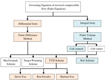
2.2 Hierarchy of CFD solver

(31)

[image:31.595.144.491.479.742.2]

starts from the governing equation of fluid motion. Figure 2.1 shows the road map in solving the flow problem by using CFD. The governing equation can be basically presented in either differential form or integral form. If the need chooses the governing equation in differential form, it may need to adopt a finite difference method (FDM) to solve that governing equation. Since the Euler equation represents the non-linear partial differential equation, a certain numerical technique needs to be introduced. With this, it will adopt particular manner of FDM for solving the Euler equation to be implemented and may also choose a MacCormack Scheme, Flux splitting Steger Warming or TVD scheme. The TVD scheme can be used according to Harten-Yee, Roe-Sweby or Davis-Yee TVD schemes. Meanwhile, if the need uses an integral form in representing the governing equation of fluid motion; it may use a finite volume method (FVM). In this respect, an idea of FVM based on cell vertex method or cell center method can be used. These two methods are basically concerned with the way the control point for each element is defined. While that, in terms of solving the non-linear partial differential equation, the method as introduced by Roe can be used. This method describes the flux of the flow variables. Hence the Roe method can also be used in the finite difference approach as well. The yellow bars and blue bars indicate the CFD code processes that have been developed in this study.

Figure 2.1: Hierarchy of CFD solver Governing Equation of inviscid compressible

flow (Euler Equation)

Differential form Integral form

Finite Difference Method

Finite Volume Method

MacCromack Scheme

Steger-Warming Scheme

TVD Scheme

Davis-Yee Roe-Sweaby Harteen -Yee

Cell centred Cell vertex

(32)

2.3 Governing equation

Basically describing the flow behaviour can be done by writing it in the form of governing equation of fluid motion. This governing equation of fluid motion can be written in differential form or in the integral form. Both forms are formulated based on three physical conservation laws. They are known as (1) conservation of mass (continuity equation), (2) conservation of linear momentum (Newton‟s second law) and (3) conservation of energy (first law of thermodynamics). The manner on how to derive the governing equation of fluid motion in differential form as well as in integral form can be obtained in various fluid mechanics text books [15-19]or CFD text books [20-25]

The governing equations of fluid motion expressed in differential form presented in vector notation and Cartesian are given in Eq. (2.1) to Eq. (2.5). The continuity equation can be written as below,

 

0

     V  

t (2.1)

In Eq. (2.1), the ρ, V and t represent the density of fluid, vector velocity and time respectively. The momentum equations in three components can be written as below,

x-component

 





xx yx zx fx

z y x x p u u

t       

                

V (2.2)

y-component

 





xy yy zy fy

z y x y p v v

t       

                 V (2.3) z-component

 





xz yz zz fz

z y x z p w w

t       

(33)

In Eq. (2.2) to Eq.(2.3) p is static pressure, τ is shear stress and f is flux vector. Meanwhile, u, v, w are the x, y, z components of the velocity. The energy equation can be written as below:

 





 





     













V f V                                                                                                                     z w y w x w z v y v x v z u y u x u z wp y vp x up z T k z y T k y x T k x q V e V e t zz yz xz zy yy xy zx yx xx  2 2 2 2 (2.5)

where  is vector operator, V is vector velocity, f is vector of body force per unit mass. It can be defined as below

z y x         

 i j k (2.6)

k

j i

Vu v w (2.7)

k j i

f  f_x  f_y  f_z (2.8)

Namely, Eq. (2.1) to Eq. (2.5) are representing the governing equation for viscous flow which considers the transport phenomena of friction and thermal conduction. These equations are known as Navier-Stokes equation.

2.4 Euler equation

If viscosity effect can be neglected in a fluid flow, the flow is considered to be non-viscous or inviscid. That means all elements of friction and thermal conduction will be neglected. As a result, the continuity in Eq. (2.1) can be written as below.

 

0

     V   t (2.9)

(34)

x-component

 





fx

x p u

u

t    

        V (2.10) y-component

 





fy

y p v

v

t    

        V (2.11) z-component

 





fz

z p w

w

t    

        V (2.12)

For energy equation in Eq. (2.5), it can be written as,

     

V f V                         _                _       z wp y vp x up q V e V e

t 2 2

2 2

(2.13)

In the above equations, Eq. (2.9) until Eq. (2.13), are known as Euler Equation. These equations can be used whether the flow problem belongs to the class of compressible flow or incompressible flow. Both may be in steady or unsteady flow conditions.

2.5 Available CFD code for air vehicle design and analysis

(35)

complemented each others. The wind tunnel result can be used to validate the CFD results, on other hand the CFD results can be used to calculate the wind tunnel wall correction factors. Other benefits offered by CFD would be that, this approach can narrow down the number of design constraints and parameters in which further detailed flow analysis can be conducted through wind tunnel tests. This means that CFD will identify some important flow regions where further study purposes will be carried out in wind tunnel tests by using some instrumented models [26].

[image:35.595.129.513.427.647.2]

Basically, the development of CFD throughout the history of Boeing Commercial Airplane in the process of producing their various types of commercial passenger aircrafts can be looked on. Figure 2.2 shows the Boeing aircraft generation and the corresponding CFD code associated with the development of these aircrafts. The Boeing 767 and Boeing 757 represent two examples of passenger type aircraft in which their aerodynamics analysis and design are obtained by using a CFD code named as PANAIR. While that, Boeing 737-300 series are using CFD code called FLO22 and TRANAIR. The aircraft Boeing 787 series as the most lastet aircraft are designed on the CFL3D OVERFLOW‟s CFD code [2].

Figure 2.2: Chronology of Boeing aircraft production [27]

(36)

[image:36.595.134.501.139.571.2]

the governing equation of fluid motion can be divided into several levels of governing equation as shown in Figure 2.3.

Figure 2.3: Hierarchy of governing equation [28]

(37)

[image:37.595.167.459.548.714.2]

called turbulence. This instability phenomenon occurs in almost all flow situations when the velocity, or more precisely, the Reynolds number, defined as the product of representative scales of velocity and length divided by the kinematic viscosity, exceeds a certain critical value. The particular form of instability generated in the turbulent flow regime is characterized by the presence of statistical fluctuations to the all flow quantities. These fluctuations can be considered as superimposed on mean or averaged values and can attain, in many situations, the order of 10% of the mean values, although certain flow regions, such as separated zones, can attain much higher levels of turbulent fluctuations. The numerical description of the turbulent fluctuations is a formidable task which puts very high demands on computer resources. As mentioned earlier, the numerical approach designed to solve the Navier-Stokes equation directly is DNS that is possible to be used for industrial applications which may become viable after 2080. The present computer capability is not yet sufficient enough to fulfil the DNS requirements. An attempt on reducing computer demand can be done through deep observation of the flow behaviour. It has been found that most flow problems have two types of turbulent fluctuations, a large and small scale fluctuations. In this respect, the large scale turbulent fluctuations are solved directly from the Navier-Stokes equation while a smaller scale is through its simplified form of the Navier-Stokes equation. Such approach is known as Large Eddy Simulations (LES). Unfortunately the implementation of this method to deal with industrial applications is still time consuming, it can be fully utilized after 2045 as shown in Figure 2.4 [1].

(38)

The third level of the governing equation of fluid motion is the Reynolds Averaged Navier-Stokes equation (RANS). This equation can be obtained through representing turbulent flow phenomena consisting of two quantities which are the average value and the fluctuated value. If the ratio between fluctuated value and the average value is small and the average value of the fluctuated quantity goes to zero for sufficient time, then the Navier-Stokes equation can be reformulated to become a RANS. However in solving this equation, it has to introduce a turbulence modelling. It is true that the spatial and temporal discretisation requirements are far less than the DNS or LES approach, but their solution are depending on the turbulence modelling invoked and also the numerical scheme in use.

RANS can be further simplified if the flow problem belongs to the class of high Reynolds number flow with the flow separation covered up in small flow domain. In this situation, it can ignore the viscous and turbulent diffusion terms in the main stream direction. Here the RANS equation becomes an equation known as Thin Shear Layer Equation. While that, if the pressure gradient in the normal direction of the body surface is equal to zero, then the RANS equation becomes a Parabolized Navier-Stokes equation.

(39)

[image:39.595.173.464.403.598.2]

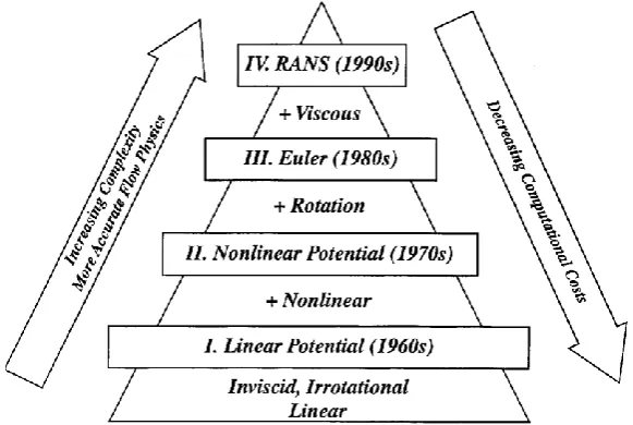
equation can be reduced to become the the continuity equation that needs to be solved. The momentum equation was initially in the form of differential equation; they can be converted to become an algebraic equation in relating the flow variables of pressure and flow velocity. The reduced form of the Euler Equation is known as a Full Potential Equation. Through a Full potential Equation further simplification can be done by considering the presence of the body immersed in the flow field creating a small perturbation into the flow field. Such flow condition makes the Full Potential Equation can be simplified to become a Prandtl-Glaured equation. This equation is applicable to the case of compressible flow at high subsonic flow or supersonic flow. In the case of transonic flow, the Full Potential Equation becomes a Transonic Small Perturbation Equation (TSP-equation). If the inviscid flow problem applied to the incompressible flow and in addition with the flow considered as irrotational flow, the Euler equation can be reformulated to become a Laplace equation. This represents the lowest level of the governing equation of fluid motion. The level of complexity of the governing equation of fluid motion is shown in Figure 2.5.

Figure 2.5: The level of complexity of the governing equation of fluid motion

2.5.1 CFD Linear potential flow equation

(40)

irrotational flow condition can be invoked. As a result, the governing equation of fluid motion can be formulated in the form of Laplace equation if the flow belongs to the class of incompressible flow or in the form of Prandtl-Glaured equation if the compressible effect needs to be taken into account. Both equations correspond with each other. The method was used for solving the Laplace equation for solving the Prandtl-Glaured equation. Initially an attempt to solve the Laplace equation is carried out by using an analytical approach. Using a complex variable, the two-dimensional (2D) flow past through shape like airfoil can be solved, so the pressure distribution along the airfoil surface can be predicted.

(41)

[image:41.595.150.493.101.344.2]

Table 2.1 List of some major Panel Method [29]

Among those Panel method as mentioned in above table, PANAIR, VSAERO and PMARC will be described further in the following sub-chapter.

2.5.1.1 PANAIR code [30]

(42)

continuous. It is also this "higher order" attribute which allows PANAIR to be used to analyse flow on arbitrary configurations. PANAIR can handle the simple configurations considered in the preliminary design phase and later serves as the "analytical wind tunnel" which can analyse the flow on the final detailed, complex configurations. In general, the aircraft surface is partitioned into several networks of surface grid points, such as a fore body network, a wing network, and so forth. The coordinates of the input grid points must be computed and entered by the user. The theoretical background on how to develop this code according to the Panel method is described in [30-33]. While that, [34-36] gives some examples on the application of the PAN AIR code for solving various flow problems

2.5.1.2 VSAERO code [37]

This code was developed by Ames Research Centre by AMI (Analytical Mechanics Inc). The code implements the surface singularity panel method using quadrilateral panel on which doublet and source singularities distributed piecewise constant form. The panel source values are directly determined by the external Neuman boundary condition controlling the normal local resultant flow. The doublet values are solved after imposing the internal Direchlet boundary condition of zero perturbation potential at the centres of the panels simultaneously. Surface perturbation velocities are obtained from the gradient of the doublet solution while field velocities are obtained by direct summation of all singularity panel contributions. In order to accommodate the ability to predict the non-linear aerodynamic characteristics, the vortex separation and vortex/surface interaction are treated in an iterative wake-shape calculation procedure, while the effects of viscosity are treated in an iterative loop coupling potential flow and integral boundary layer calculations. The user manual on how to use the VSAERO Code including its theoretical back ground can be referred to [32, 38, 39].

2.5.1.3 PMARC [40]

(43)

of Ames Research Centre”. Basically PMARC represents the extension of VSAERO code. This computer code has the same capabilities as the VSAERO codes; it has several advanced features such as the ability in dealing with the internal flow model, a simple jet wake model, and a time-stepping wake model. In addition to that, the data management within the code has been optimized by the use of an adjustable size arrays for rapidly changing the size capability of the code, reorganization of the output file and adopting a new plot file format. The Panel method which had been used in developing PMARC code may be referred to [41, 42].

2.5.2 Potential flow equation

Basically, there are three conservative formulations used for inviscid transonic flow. They are followed by transonic small-disturbance equation, full potential equation and Euler equation for the exact inviscid formulation. Transonic small-disturbance is suitable to solve transonic flow with simple geometry. Transonic small-disturbance has been solved for lifting, sweat-wings and simple wing-fuselage combination. Meanwhile, the full potential for complex body includes bodies of revolution, asymmetric and planar inlet nacelles and yawed [43]. The solver for transonic-small disturbance has been developed in the early 1970s by Murman and Cole by using concept within subsonic regions and backward differences within supersonic regions. Then the modification of Murman and Cole scheme has been used to solve full potential flow equation [4].

2.5.2.1 FLO22 & FLO27 [5]

(44)

2.5.2.2 TRANAIR [44]

This code was also developed by Boeing Company and NASA. This code has been used heavily on commercial transport designs since the 777 – 200. TRANAIR code development began under contract with NASA as a feasibility study in 1984. The technology to analyze transonic flow with a uniform orthogonal field grid was developed under this initial contract. Further development under a second NASA contract led to the development of grid refinement techniques. Today TRANAIR code is a fully functional analysis and design tool with continuous development in design, adaptive grid refinement, coupled boundary layer and design capability

2.5.3 Euler equation

The highest level of the inviscid flow is Euler equation. For many practical aerodynamic applications, this equation is relatively accurate for representing the flow field which includes both rotational and discontinuous (shock) phenomena in the flow and providing an excellent approximation for lift induced drag and wave drag. Furthermore, a robust Euler solver is an essential part of any Navier-Stokes solver. In addition to this, Euler equations promised to provide more accurate solutions of transonic flows.

The Euler equation was used by Jameson in developing computer code for solving a 3D flow problem named FLO57 code in 1981. It was used to develop other codes called a MGAERO code. MGAERO code is unique in being a structured Cartesian mesh code. Besides that, Jameson also developed the AIRPLANE code which made use of unstructured tetrahedral grids. In the 2D, Drela and Giles developed the ISES code for airfoil design and analysis. This code first became available in 1986 and has been further developed to design, analyze and optimize single or multi-element airfoils, also known as MSES code.

2.5.3.1 FLO57 [6]

(45)

REFERENCES

1. Tinoco, E. N. The Impact of High Performance Computing and Computational Fluid Dynamics on Aircraft Development. 20th Anniversary Dinner &

Symposium CASC. Washinton, DC: Coalation for Academic Scientific

Computation. 2009.

2. Johnson, F.T., Tinoco, E. N., & Yu, N. J. Thirty years of development and application of CFD at Boeing Commercial Airplanes, Seattle. Computers &

Fluids. 2005. 34: 1115-1151.

3. Hess, J. L. & Smith, A. M. Calculation of non-lifting potential flow about arbitrary three-dimensional bodies: DTIC Document. 1962.

4. Cole, J. D. & Murman, E. M. Calculation of plane steady transonic flows.

AIAA Journal. 1971. 9: 114-121.

5. Jameson, A. & Caughey, D. A. Caughey. A finite volume method for transonic potential flow calculations. AIAA Paper. 1977. 635.

6. Jameson, A. & Schmidt, W. and Turkel, E. Numerical solutions of the Euler equations by finite volume methods using Runge-Kutta time-stepping schemes.

AIAA Paper. 1981. 1259.

7. Jameson, A. & Schmidt, W. and Turkel, E. Numerical solution of the Euler equations by finite volume methods using Runge Kutta time stepping schemes.

14th Fluid and Plasma Dynamics Conference. American Institute of

Aeronautics and Astronautics. 1981.

8. Drela, A. Newton solution of coupled viscous/inviscid multielement airfoil flows. 21st Fluid Dynamics, Plasma Dynamics and Lasers Conference. American Institute of Aeronautics and Astronautics. 1990.

(46)

10. Jameson, A., Martinelli, L. & Vassberg, J. Using computational fluid dynamics for aerodynamics - a critical assessment. Proceedings of ICAS. 2002: 1-10. 11. Godunov, S. A. difference method for numerical calculation of discontinuous

solutions of the equations of hydrodynamics. Matematicheskii Sbornik. 1959. 89: 271-306.

12. Roe, P. L. Approximate Riemann solvers, parameter vectors, and difference schemes. Journal of Computational Physics. 1981. 43: 357-372,.

13. Harten, A. High resolution schemes for hyperbolic conservation laws. Journal of

Computational Physics. 1983. 49: 357-393.

14. Harten, A. On the symmetric form of systems of conservation laws with entropy.

Journal of Computational Physics. 1983. 49:151-164.

15. Subrahmaniyam, S. Fluid mechanics. New Delhi. Capital Publishing. 2007. 16. Munson, B. R. Fundamentals of fluid mechanics (6th ed.). Hoboken NJ. Wiley.

2010.

17. Munson, B. R. Fluid mechanics (10th ed.). Hoboken, NJ. Wiley. 2013. 18. White, F. M. Fluid Mechanics. Boston. McGraw-Hill,.2008.

19. Janna, W. S. Introduction to fluid mechanics. Boca Raton. CRC Press. 2010. 20. Blazek, J. Computational Fluid Dynamics: Principles and Applications. Elsevier.

2005.

21. Hoffman, K. A. & Chiang, S. T. Computational Fluid Dynamicsvol. II. (4th ed). USA: www.EESbooks.com. 2000.

22. Hoffman, K. A. &Chiang, S. T. Computational Fluid Dynamics vol. I. (4th ed.). USA: www.EESbooks.com. 2000.

23. Chung, T. J. Computational fluid dynamics. Cambridge university press, 2010. 24. Tannehill, J. C. & Anderson, D. A. & Pletcher, R. H. Computational Fluid

Mechanics and Heat Transfer (2nd ed). United State of America. Taylor &

Francis. 1997.

25. Anderson, J. D. Computational Fluid Dynamics : The Basic with Application. New York. McCraw-Hill. 1995.

(47)

27. Jameson, A. Computational Past, Present and Future. AMS Seminar Series.

Moffett Field, CA: 2012.

28. Hirsh, C. Numerical Computation of Internal and External Flows (2nd ed). Great Britian. Elsevier. 2007.

29. Henne, P. A. Applied computational aerodynamics. Washington, DC. American Institute of Aeronautics and Astronautics. 1990.

30. Magnus, A. E. & Epton, M. A. PAN AIR-A Computer Program for Predicting Subsonic or Supersonic Linear Potential Flows about Arbitrary Configurations Using a Higher Order Panel Method. Volume I. Theory Document (Version 1.0). NASA. CR-3251. 1980.

31. Sidwell, K. W., Baruah, P. K.,Bussoletti, J. E., Medan,T. R. & Conner, S. PAN AIR - A Computer Program for Predicting Subsonic or Supersonic Linear Potential Flows About Arbitrary Configurations Using A Higher Order Panel Method, Vol. II. User's Manual (Version 1.0). NASA. 1980.

32. Larry, L. E. Panel Method - An Introduction. Ames Research Centre, Moffett Field, California. Nasa Technical Paper 2995.1990.

33. Derbyshire, T. & Sidwell, K. W. PAN AIR Summary Document, (Version 1.0). NASA. 1982.

34. Alexander, J. I. D., Johnson, F. T. & Freeman, L. M. Application of a higher order panel method to realistic supersonic configurations. Journal of

Aircraft.1980. 17: 38-441980.

35. Lee, K. D. Numerical Simulation of the Wind Tunnel Environment by a Panel Method. AIAA Journal, 1981. 19: 470-475.

36. Chen, A. W. & Tinoco, E. N. PAN AIR applications to aero-propulsion integration. Journal of Aircraft. 1984. 21:161-167.

37. Maskew, B. Prediction of Subsonic Aerodynamic Characteristics: A Case for Low-Order Panel Methods. Journal of Aircraft. 1982. 19: 157-163.

38. Maskew, B. Program VSAERO theory Document: a computer program for

calculating nonlinear aerodynamic characteristics of arbitrary configurations .

4023. NASA. 1987.

(48)

40. Ashby, D. L., Dudley, M. R. & Iguchi, S. K. Development and validation of an

advanced low-order panel method: NASA, Ames Research Center. 1988.

41. Hess, J. L. Calculation of potential flow about arbitrary three-dimensional lifting bodies. DTIC Document. 1972.

42. Ashby, D. L., Dudley, M. R., Iguchi,S. K., Browne, L. & Katz, J. Potential Flow Theory and Operation Guide for the Panel Code PMARC 12. NASA, Ames Research Center. 1992.

43. Caughey, D. A. & Jameson, A. Numerical Calculation of Transonic Potential Flow about Wing-Body Combinations. AIAA Journal. 1979. 17: 175-181.

44. Samant, S., Bussoletti, J., Johnson, F., Burkhart, Everson, R., Melvin, B. R., Young, D., Erickson, L. & Madson, M.TRANAIR - A computer code for transonic analyses of arbitrary configurations. 25th AIAA Aerospace Sciences

Meeting: AIAA. 1987.

45. Giles, M., Drela, M. & Thompkins, W. J. R. Newton solution of direct and inverse transonic Euler equations. 7th Computational Physics Conferene: AIAA. 1985.

46. Jameson,A., Baker, T. & Weatherill, N. Calculation of Inviscid Transonic Flow over a Complete Aircraft. 24th Aerospace Sciences Meeting: AIAA. 1986.

47. Tidd, D., Strash, D. Epstein, B., Luntz, A., Nachshon, A. & Rubin, T. Application of an efficient 3-D multigrid Euler method (MGAERO) to complete aircraft configurations. 9th Applied Aerodynamics Conference: AIAA. 1991. 48. Mohamad, M. A. H., Basri, S. & Basuno, B. One-dimensional high-order

compact method for solving Euler equations. 2013.

49. Zulkafli, B., Fadhli, M. Omar, A. A. E. & Asrar W. Numerical analysis of FDV method for one-dimensional Euler equations. 2012: 1-6.

50. Wahi, N. & Ismail, F. Numerical shock instability on 1D Euler equations. AIP

Conference Proceedings. 2013. 1522: 376-383.

51. Roslan, N. K. H. & Ismail, F. Evaluation of the entropy consistent euler flux on 1D and 2D test problems. The 4th International Meeting Of Advances In

Thermofluids. 2012: 671-678.

52. Ghuanghui, H. Numerical simulations of the steady Euler equation on

(49)

53. Botte,G. G., Ritter, J. A. & White, R. E. Comparison of finite difference and control volume methods for solving differential equations. Computers &

Chemical Engineering. 2000. 24: 2633-2654.

54. Terzi, D. V., Linnick, M., Seidel, J. & Fasel, H. Immersed boundary techniques for high-order finite-difference methods. 15th AIAA Computational Fluid

Dynamics Conference: AIAA. 2001.

55. Thomas, P. High Order Accurate Finite-Difference Methods: as seen in OVERFLOW. 20th AIAA Computational Fluid Dynamics Conference: AIAA. 2011.

56. Ray, H., Nallasamy, M. & Scott, S. A Method for the Implementation of Boundary Conditions in High-Accuracy Finite-Difference Schemes. 43rd AIAA

Aerospace Sciences Meeting and Exhibit: AIAA. 2005.

57. Mead H. R. & Melnik. R. E. GRUMFOIL: A Computer Code for the Viscoues Transonic Flow Over Airfoils. NASA CR-3806. 1985.

58. Yee, H. C.Upwind and symmetric shock-capturing schemes. NASA Ames Research Center; Moffett Field, CA, United States NASA-TM-89464. 1987. 59. Harten, A. On a Class of High Resolution Total-Variation-Stable

Finite-Difference Schemes. SIAM Journal on Numerical Analysis. 1984. 21:1-23. 60. Yee, H. C. & Kutler, P. Application of second-order-accurate total variation

diminishing (TVD) schemes to the Euler equations in general geometries. NASA Ames Research Center; Moffett Field, CA, United States. NASA-TM-85845. 1983.

61. Yee, H. C., Warming, R. F. & Harten, A. Implicit total variation diminishing (TVD) schemes for steady-state calculations. 6th Computational Fluid Dynamics

Conference Danvers. 1983.

62. Yee, H. C., Warming, R. F. & Harten, A. Implicit total variation diminishing (TVD) schemes for steady-state calculations. Journal of Computational Physics.

1985. 57: 327-360.

63. Yee, H. C. & Harten, A. Implicit TVD schemes for hyperbolic conservation laws in curvilinearcoordinates. AIAA JournaL. 1985. 25:

(50)

65. Van Leer, B. Towards the ultimate conservative difference scheme. V. A second-order sequel to Godunov's method. Journal of Computational Physics. 1979. 32: 101-136.

66. Sohn, S.-I. A new TVD-MUSCL scheme for hyperbolic conservation laws.

Computers & Mathematics with Applications. 2005. 50: 231-248.

67. Davis, S. F. A Simplified TVD Finite Difference Scheme via Artificial Viscosity.

SIAM Journal on Scientific and Statistical Computing. 1987. 8: 1-18.

68. Kroll, N., Gaitonde, D. & Aftosmis, M. A systematic comparative study of several high resolution schemes for complex problems in high speed flows. in

29th Aerospace Sciences Meeting: AIAA. 1991.

69. Chen, M.-H., Hsu, C.-C. & Shyy, W. Assessment of TVD schemes for inviscid and turbulent flow computation. International Journal for Numerical Methods in

Fluids. 1991. 12: 161-177.

70. Qureshi K. R. & Lee C. H. Behavior Of Tvd Limiters On The Solution Of Non-Linear Hyperbolic Equation. Modern Physics Letter. 2005. 19: 1507-1510. 71. Chang,Y. L. Development of a CFD code using TVD schmes and advanced

turbulence models for incompressible flow simulations. Thesis Ph.D. Michigan

Technological University; 1997.

72. Glaister, P. Flux difference splitting for the Euler equations in one spatial co-ordinate with area variation. International Journal for Numerical Methods in

Fluids. 1988. 8: 97-119.

73. Glaister, P. A weak formulation of Roe's scheme for two-dimensional, unsteady, compressible flows and steady, supersonic flows. Computers & Mathematics

with Applications, 1995. 30: 85-93.

74. Abgrall, R. M. An extension of Roe's upwind scheme to algebraic equilibrium real gas models. Computers & Fluids, 1991. 19: 171-182.

75. Mottura, L., Vigevano, L. & Zaccanti, M. An Evaluation of Roe's Scheme Generalizations for Equilibrium Real Gas Flows. Journal of Computational

Physics. 1977. 138: 354-399.

(51)

77. Anderson, W. K., Thomas, J. L. & Van Leer, B. Comparison of finite volume flux vector splittings for the Euler equations. AIAA Journal. 1986. 24: 1453-1460.

78. Jameson, A. Requirements and trends of computational fluid dynamics as a tool for aircraft design. Proceedings of the 12th NAL symposium on aircraft

computational aerodynamic. Tokyo, Japan. 1994.

79. Maciel, E. S. G. TVD Algorithms Applied to the Solution of the Euler and Navier-Stokes Equations in Three-Dimensions. WSEAS Transactions on

Mathematics.2012. 11: 546-572.

80. Maciel, E. S. G. Explicit and Implicit TVD and ENO High Resolution Algorithms Applied to the Euler and Navier-Stokes Equations in Three-Dimensional Turbulent Results. 2013.

81. Shigeki, H., Justin, A., Klaus, H. &Ramesh, A. Development of a modified Runge-Kutta scheme with TVD limiters for the ideal 1-D MHD equations. 13th

Computational Fluid Dynamics Conference. 1997.

82. Shigeki, H., Klaus, H. & Justin, A. Development of a modified Runge-Kutta scheme with TVD limiters for the ideal two-dimensional MHD equations. 36th

AIAA Aerospace Sciences Meeting and Exhibit: American Institute of

Aeronautics and Astronautics. 1998.

83. Anderson, J. D. Introduction to flight. New York: McGraw-Hill. 2015.

84. Harris, C. D. Two-dimensional aerodynamic characteristics of the NACA 0012 airfoil in the Langley 8 foot transonic pressure tunnel. 1981.

85. Gregory, N. & O'Reilly, C. L. Low-Speed aerodynamic characteristics of NACA 0012 aerofoil section, including the effects of upper-surface roughness

simulating hoar frost: HM Stationery Office. 1973.

86. Hess, R. W. Unsteady pressure measurements on a supercritical airfoil at high Reynolds numbers. 1989.