Journal of Chemical and Pharmaceutical Research, 2014, 6(3):1233-1238
Research Article
CODEN(USA) : JCPRC5
ISSN : 0975-7384
Distribution network design in battlefield environment with loss consideration
Ji Ren
1*, Yue-Jin Tan
1, Xiao-Lei Zheng
21Science and Technology on Information Systems Engineering Laboratory, National University of Defense Technology, Changsha, P.R. China
2
Lagistic Command College, Beijing, China
_____________________________________________________________________________________________
ABSTRACT
We study the distribution network design problem in a battlefield environment. The problem is to decide where to locate the distribution nodes and which distribution nodes or supply nodes the combat units are allocated to minim-ize the total setup cost and transportation cost. Some commodities would be destroyed by the enemy during the dis-tribution process, and the loss quantity is assumed to follow a function of the exposure time in the disdis-tribution process. An Integer Programming model is proposed to formulate the problem, which is solved by Lagrangian heu-ristic algorithm. One hundred numerical examples including up to 20 supply nodes, 80 distribution nodes and 400 combat nodes are randomly generated based on data investigated from military wars and games, and all of them are used to test the solution approach. Computational results show that the algorithm can present very good near-optimal solution within short computational time.
Key words: Battlefield supply, network design, integer programming, Lagrangian relaxation
_____________________________________________________________________________________________
INTRODUCTION
The successful completion of combat missions depends heavily on the reliability and availability of the military lo-gistic support system, as combat units can only exert all their power when they receive the right support commodi-ties in the right place, at the right time, and in the right quantity [1-3]. In the military history, the backside logistic support system is always one of the most important strategic targets that are attacked by enemies. In recent decades, as the application and generalization of information technologies, more and more reconnaissance equipments with high precision and long-distance attacking weapons are developed and equipped in army [4-6]. Therefore, in current wars, the military logistic systems in battlefield suffer more frequent and severe attack from the enemy, which cause much loss when the commodities are transported from backside base to the front combat units.
Recent wars, such as the War in the Persian Gulf, and the Iraq War, have shown that military logistics face many new challenges in modern battlefield, which include frequent and small delivery bathes, higher agility, and much shorter response time and so on. Many new logistic theories are developed to cover these new requirements, like Focused Logistics [7-10], Sense and Response Logistics [11-13]. To support the implement of these new theories, effective and efficient distribution networks are required.
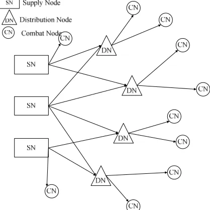
Fig. 1 The distribution network in the battlefield
In the proposed distribution network in Fig. 1, it is assumed that commodities in SNs are safe and can not be de-tected by the enemy, as the backside military bases are usually underground. When commodities are sent out and transported to CNs, they may be detected and attacked by the enemy during the distribution time, which would cause some losses. The more time of the commodities consume in the distribution process, the more quantity would be destroyed by the enemy.
The proposed problem can be viewed as a two-layer facility location problem. As an important area, many achieve-ments have been obtained on distribution network design and facility location problem [14-15]. But fewer models are developed specially for distribution systems in the battlefield environment. Gue investigates a sea-based logistic system, and develops a multi-period, facility location and material flow model for the system. The proposed model can be used to construct the land-based distribution system over time to support a given battle plan with minimum inventory. Toyoglu et al. study an ammunition distribution problem in the battlefield and develop a novel three-layer commodity-flow location routing model that helps distribute multiple products, respects hard time windows, to the combat units. As far as we know, there is no work considering the loss caused by attacks from the enemy in the de-sign of distribution systems [16-20].
The organization of this paper is as follows. In section 2, the distribution network design problem is formulated into Integer Programming model. The solution approach for the problem is developed in section 3 and the computational results are discussed in section 4. We conclude the paper in section 5.
MODEL FORMULATION
In the battlefield distribution network, each supply node supplies a different commodity and can satisfy all the de-mand from CNs. In practical war, military bases usually supply multiple kinds of commodities. Thus, some of the supply nodes here are virtual nodes. The commodities are first transported to the DNs from the SNs and then deli-vered to the CNs, and they can be also sent to the CN directly from the SN if the distance between them is close enough. The commodities form the same SN can either be delivered form SN or through one DN, but not from both or through more than one DN.
The following notations are used in the MIP model:
i=1,2,…,I: index of SNs
j=1,2,…,J: index of potential DNs k=1,2,…,K: index of CNs
Parameters:
ci = the unit cost of commodity i
dik = demand for commodity i at combat node k
tdj = the dwell time at DN j
tpdij = the transportation time from SN i to DN j
tprik = the transportation time from SN i to CN k
cpdij = the cost of transporting per commodity from SN i to DN j
cdrjk = the cost of transporting per commodity from DN j to CN k
cprik = the cost of transporting per commodity directly from SN i to CN k
fj = the setup cost of DN j
The dwell time at DN j, tdj, is the overall time spent on the DN j from receiving the commodities until sending out them, which includes the unloading time, the sorting time, the upload time and so on.
The decision variables are defined as follows:
Xijk 1 if the demand of CN k are transported from SN i through DN j, otherwise 0;
Yik 1 if the demand of CN k are transported from SN i directly, otherwise 0
Zj 1 if DN j is setup, otherwise 0.
Here we make the assumption that the loss rate of commodities transported from SNs to CNs depends on the deli-very time from SNs to CNs, and the longer of the exposure time, the more commodities would be destroyed by the enemy. Therefore the excepted quantity that can safely arrived at the combat is described as follows,
DE=DIg(t) (1)
where DE is the excepted quantity that can safely arrived at the cambat node, DI is the initial quantity sent out from the supply node, t is the total exposure time, and g(t) is a nonincreasing function of the exposure time, which satis-fies 0<g(t) ≤1. Let tijk=tpdij+tdj+tdrjk= the exposure time from SN i to CN k through DN j. tik=tprik= the exposure time from SN i to CN k directly. Then, the required initial quantities sent out from supply nodes in different ways are dik/g(tijk) or dik/g(tik).
In fact the presented distribution network design problem can be viewed as a special case of two-level facility loca-tion problem. The mathematical optimizaloca-tion model for the problem is formulated as follows.
Min
1 1 1 1 1 1
(
)
(
)
( )
( )
I J K I K J
ik ijk ik ik
i ij jk i ik j j
i j k i k j
ijk ik
d X
d Y
c
cpd
cdr
c
cpr
f Z
g t
g t
= = = = = =
+
+
+
+
+
∑∑∑
∑∑
∑
(2)
s.t. 1
1
,
J ijk ik jX
Y
i k
=
+ =
∀
∑
(3)
, ,
ijk j
X
≤
Z
∀
i j k
(4){ }
,
,
0,1
, ,
ijk ik j
X
Y Z
∈
∀
i j k
(5)
The objective function is to minimize the overall cost. Constraint (3) ensures that the demand of CN k from SN i is satisfied by shipment through one DN or by shipment directly from the SN, but not by both. Constraint (4) ensures that the commodities can only be transported through the DN which has been opened. Constraint (5) is the integer restriction.
SOLUTION ALGORITHM
To introduce conveniently, we note that
a
ijk=
(
c
ik+
cpd
ij+
cdr d
jk)
ikg t
( )
ijk andb
ik=
(
c
ik+
cpr d
ik)
ikg t
( )
ik .The relaxed problem can be obtained by relaxing the constraint set (3).
Min
1 1 1 1 1 1 1 1 1
(1
)
I J K J I K I K J
ijk ijk j j ik ik ik ijk ik
i j k j i k i k j
a X
f Z
b Y
λ
X
Y
= = = = = = = = =
+
+
+
−
−
∑∑∑
∑
∑∑
∑∑
∑
Subject to (4) and (5). Then the relaxed problem is decomposed into independent subproblems.
1) Subproblem for SN i
Min
1
(
)
K
ik ik ik
k
b
λ
Y
=
−
∑
Yik=1; Otherwise, set Yik to be zero.
2) Subproblem for DN j
Min
1 1 1 1
(
)
I K I K
j j ik ijk ijk ik
i k i k
f Z
λ
a
X
λ
= = = =
−
∑∑
−
+
∑∑
,Subject to (4) and Xijk, Zj ∈{0,1}, ∀i,j,k. The solution procedure of the second subproblem is as follows:
Step 0 (Initialization):
Zj=0; Xijk=0 Step 1 Iteration For i=1 to I For k=1 to K If λik−aijk≥0 Then Xijk=1 end for
end for.
Step 2 Judge
If
1 1
(
)
I K
ik ijk ijk j j
i k
a
X
f Z
λ
= =
−
≥
∑∑
then Zj=1 else set all Xijk=0.
Here we use subgradient algorithm to obtain an upper bound for the problem. The main steps of the algorithm are as follows:
Step 0 Initialization
Let LR be the objective value of the Lagrangian relaxation problem, and set LR=0. Let UB be the upper bound of the problem, and set UB= +∞.
Let LB be the lower bound of the problem, and set LB= −∞. Set λik=bik+1, and α=2.
Step 2: Update lower bound If LR>LB, then LB=LR.
Step 3: Update upper bound
If the relaxed solution satisfies constraint and its corresponding objective function value is
F
′ <
UB
, then letUB
=
F
′
.Step 4: Calculate new step size
Let
(1
ijk ik)
2i k j
norm
=
∑ ∑
−
∑
X
−
Y
If norm>0
(
) /
stepsize
=
α
UB
−
LR
norm
Otherwise,
stepsize
=
stepsize
/ 2
.Step 1 Solve subproblems
Given λik, solve subproblems for SN i and DN j, then obtain a new bound LR.
Step 2 Update lower bound If LR>LB, let LB=LR.
Step 3 Update upper bound
Step 4 Calculate new step size
Let norm=
(1
ijk ik)
2i k j
X
Y
−
−
∑ ∑
∑
If norm>0
stepsize=α(UB−LR)/norm else stepsize=stepsize/2.
Step 5 Update multipliers
).
1
(
*
ikj ijk ik
ik
=
λ
−
stepsize
−
∑
X
−
Y
λ
Step 6 Stopping criteria
If the number of iterations > Ni or the max gap of λik between two coterminous iteration is less than ε,
then STOP, else GOTO step 1. Ni and ε is defined by user according requirement, in our problem
Ni=200 and ε=0.01.
Here we use a heuristic algorithm to obtain a feasible solution for the problem from the bound given by the subgra-dient algorithm. The main steps of the heuristic algorithm are as follows:
Step 0 Find an infeasible constraint and initialize
Find an infeasible pair (i, k) which
1
1
Jijk ik j
X
Y
=
+
≠
∑
,and let Xijk=0(∀j), Yik=0
Step 1 Find a node to allocate
Find a best DN j among current open DNs which
B
J=
min
{
a
ijkZ
j=
1
}
.If BJ<bik, allocate CN k to DN j and XiJk=1, else allocate CN k to SN i and Yik=1
Step 2 Judge
If there are no infeasible pairs, STOP, else GOTO step 0.
RESULTS AND DISCUSSION
The presented model and algorithm are tested on randomly generated numerical examples. And the computational experience for all examples is conducted on the IBM T420 laptop with Windows XP (Intel® Core™2 Duo CPU, 2GB of RAM).
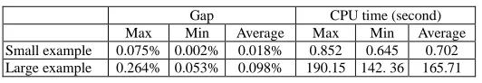
[image:5.595.174.440.674.720.2]In order to test the robust of the solution algorithm, fifty examples with the size of 5 SNs, 20 DNs and 50 CNs are generated, and fifty examples with the size of 20 SNs, 80 DNs and 400 CNs are generated. All these examples are randomly generated and solved by our solution approach. The computational performance is summarized in Table 1. The gap represents the percentage error between the feasible lower bound obtained by the heuristic algorithm and the upper bound obtained by the subgradient algorithm. From Table 1 we can see the Lagrangian heuristic approach works very well for all the examples and can present very good solution in short CPU time. Here we should also note that the results in table 1 are obtained in 200 iterations and better results can be obtained with more iteration.
Table 1 computational performance of the algorithm
Gap CPU time (second) Max Min Average Max Min Average Small example 0.075% 0.002% 0.018% 0.852 0.645 0.702 Large example 0.264% 0.053% 0.098% 190.15 142. 36 165.71
CONCLUSION
destroy of commodities by the attacks from the enemy. The problem is formulated as an Integer Programming mod-el. An efficient Lagrangian heuristic algorithm is developed to solve the problem. Fifty numerical examples for networks including 5 SNs, 20 DNs and 50 CNs, and fifty examples including 20 SNs, 80 DNs and 400 CNs are used to test the model and the solution approach. Computational performance analysis shows that the algorithm can present near optimal solutions for all examples in short CPU. In this paper, the loss function of commodities is as-sumed to constant and known, while in practical wars it is usual uncertain. Therefore, the stochastic situation of the distribution network design problem in battlefield environment would be a valuable extension to this study.
REFERENES
[1]Klose A and Drexl A, Eur J Oper Res, 2005: 162(1): 4-29
[2]Xing LN, Chen YW and Yang KW, Appl Soft Comput, 2010, 10(3): 888-896 [3]ReVelle CS, Eiselt HA, Eur J Oper Res, 2008, 184: 817-848
[4]Ambrosino D and Scutellá MG, Eur J Oper Res, 2005, 165: 610-624 [5]Geoffrion A and Powers RF, Interfaces, 1995, 25: 105-127
[6]Şahina G and Süral H, Comput Oper Res, 2007, 34: 2310-2331
[7]Xing LN, Chen YW and Yang KW, Comput Optim Appl, 2011, 48(1): 139-155 [8]Goetschalckx M, Carlos JV and Dogan K, Eur J Oper Res, 2002, 143: 1-18 [9]Erenguc SS, Simpson NC and Vakharia AJ, Eur J Oper Res, 1999, 115: 219-236 [10]Vidal JC and Goetschalckx M, Eur J Oper Res, 1997, 98: 1-18
[11]Gue KR, Comput Oper Res, 2003, 30: 367-381
[12]Toyoglu H, Karasan OE and Kara BY, Nav Res Logist, 2011, 58: 188-209
[13]Xing LN, Rohlfshagen P, Chen YW, IEEE T Evolut Comput, 2010, 14(3): 356-374 [14]Sun K, Chen YW, Wang P, Res J Chem Environ, 2012, 16(S1): 56-61
[15]Xing LN, Rohlfshagen P, Chen YW, IEEE T Syst Man Cy B, 2011, 41(4) 1110-1123 [16]Yao F, Xing LN, Disa Adv, 2012, 5(4), 1341-1344
[17]Li JF, Xing LN, Disa Adv, 2012, 5(4), 726-729
[18]Xing LN, Yang KW, Chen YW, Eur J Oper Res, 2009, 197(2): 830-833 [19]Ma WJ, Jiao BQ, Res J Chem Environ, 2012, 16(S1): 137-139