www.hydrol-earth-syst-sci.net/18/3777/2014/ doi:10.5194/hess-18-3777-2014
© Author(s) 2014. CC Attribution 3.0 License.
Robust global sensitivity analysis of a river management model to
assess nonlinear and interaction effects
L. J. M. Peeters1, G. M. Podger2, T. Smith2, T. Pickett3, R. H. Bark4, and S. M. Cuddy2 1CSIRO Land and Water, Water for a Healthy Country Flagship, Adelaide, Australia 2CSIRO Land and Water, Water for a Healthy Country Flagship, Canberra, Australia 3CSIRO Land and Water, Water for a Healthy Country Flagship, Brisbane, Australia 4CSIRO Ecosystem Sciences, Water for a Healthy Country Flagship, Brisbane, Australia
Correspondence to: L. J. M. Peeters ([email protected])
Received: 19 February 2014 – Published in Hydrol. Earth Syst. Sci. Discuss.: 25 March 2014 Revised: 1 August 2014 – Accepted: 1 September 2014 – Published: 29 September 2014
Abstract. The simulation of routing and distribution of wa-ter through a regulated river system with a river management model will quickly result in complex and nonlinear model behaviour. A robust sensitivity analysis increases the trans-parency of the model and provides both the modeller and the system manager with a better understanding and insight on how the model simulates reality and management operations. In this study, a robust, density-based sensitivity analysis, developed by Plischke et al. (2013), is applied to an eWa-ter Source river management model. This sensitivity analy-sis methodology is extended to not only account for main effects but also for interaction effects. The combination of sensitivity indices and scatter plots enables the identifica-tion of major linear effects as well as subtle minor and nonlinear effects.
The case study is an idealized river management model representing typical conditions of the southern Murray– Darling Basin in Australia for which the sensitivity of a vari-ety of model outcomes to variations in the driving forces, in-flow to the system, rainfall and potential evapotranspiration, is examined. The model outcomes are most sensitive to the inflow to the system, but the sensitivity analysis identified minor effects of potential evapotranspiration and nonlinear interaction effects between inflow and potential evapotran-spiration.
1 Introduction
Water managers rely heavily on models to predict future wa-ter availability, optimize wawa-ter use and evaluate wawa-ter man-agement strategies in order to find a balance between envi-ronmental, social and economic demands on the system. It is therefore crucial to be aware of the ability of a model to capture the dynamics of the hydrological cycle relevant to the water management question. In recent decades, address-ing this issue has been the focus of much research in hydro-logical model calibration and predictive uncertainty analysis (Gupta et al., 2012).
For a modeller, to arrive at a “well”-calibrated model or to produce sensible and robust prediction intervals, it is es-sential to have a thorough understanding of how the hydro-logical system works and how this system is represented in the model – how a variation in parameters, boundary condi-tions or driving forces will affect the prediction of interest. The knowledge gained from such sensitivity analysis is not only of relevance during model development, it also provides added value to the model as it can focus management and monitoring to those aspects of the system and model that are most important to the management of water resources (Saltelli et al., 2008). Additionally, discussing model sensi-tivities with stakeholders will remove the notion of the model being a “black box” and can provide stakeholders with a better appreciation of the accuracy of the model, which has proven to be a key aspect of adoption of model results by management (Patt, 2009; Bark et al., 2013).
3778 L. J. M. Peeters et al.: Robust global sensitivity analysis of a river management model in the development of basin-wide water allocation plans. As
these plans directly affect the livelihood of people and the health of ecosystems, it is essential that the models under-pinning these plans have wide support and are robust. It is therefore essential that practitioners have a set of tools for sensitivity analysis available, tailored to the needs of water allocation modelling. The most straightforward sensitivity analysis technique is One-At-a-Time (OAT) sensitivity anal-ysis in which one model aspect is changed while the oth-ers are fixed. The sensitivity of the model output to varia-tion of the tested parameter is proporvaria-tional to the gradient of the response surface. This is formalized in gradient-based calibration routines, such as Levenberg–Marquardt optimiza-tion. Examples of such OAT sensitivity analysis are Doherty and Hunt (2009), Foglia et al. (2009), Castaings et al. (2009) and Peeters et al. (2011). This methodology is attractive as it requires a very limited number of model runs, about two or three model runs per parameter evaluated, and, as long as the model behaves linearly, parameter interaction effects can be explored (Hill and Tiedeman, 2007). Saltelli and Annoni (2010) highlight that OAT sensitivity analysis only provides reliable and robust results if it can be shown that the model behaviour is linear. This condition is seldom satisfied for hy-drological models or even known before a sensitivity anal-ysis. The Elementary Effects method (Campolongo et al., 2007) is more robust against nonlinearity in the model be-haviour, whilst still being frugal in the number of model runs. Global sensitivity analysis techniques however do not re-quire the model behaviour to be linear (Saltelli et al., 2008). The most straightforward global sensitivity analysis is ei-ther random or density-based sampling of parameter space and visualizing scatter plots of the parameter value against the prediction of interest (Wagener and Kollat, 2007; Peeters et al., 2013). Variance-based methods, such as Sobol’ sen-sitivity analysis (Saltelli and Annoni, 2010; Nossent et al., 2011), use a scheme of structured resampling of a random base sampling to decompose the variance of the metric of interest into the main effects of a parameter and interaction effects of other parameters.
The main drawback of variance-based methods is that it assumes that the entire effect of a parameter can be summa-rized by the variance (Borgonovo, 2007; Borgonovo et al., 2011). Variance-based sensitivity indices will therefore be less reliable if the response to a parameter has a skewed or multi-modal distribution. Density-based sensitivity analysis techniques attempt to account for this by incorporating the entire distribution of the response of a prediction of interest in the metric in a way that does not require any assumptions on the shape of the distribution. The methodology suggested by Plischke et al. (2013) implements such a density-based sensitivity analysis technique which is independent of the pa-rameter sampling scheme. This has the added benefit that as no model runs need to be devoted to the resampling of a base sampling, more computing resources can be directed to ex-ploration of parameter space.
The goal of this study is to apply a density-based sensi-tivity analysis in a river management modelling context to assess its capability to identify and quantify nonlinear effects and to extend the methodology to account for interaction ef-fects. An idealized, hypothetical river management model implemented in the eWater Source platform (Welsh et al., 2013) serves as testing platform to assess the ability of the sensitivity analysis methodology to quantify the influence of a small number of forcing variables upon a variety of model outcomes.
The next section presents the theoretical background and numerical implementation of the Plischke et al. (2013) global sensitivity analysis method. The river management model is briefly introduced before presenting the results of the sensi-tivity analysis and summarizing the findings in the discussion and conclusion sections.
2 Methods
The sensitivity analysis introduced in Plischke et al. (2013) provides a robust, global density-based sensitivity analysis, independent of sampling strategy. This section provides a short summary of this methodology. For a detailed overview the interested reader is referred to Plischke et al. (2013).
ConsiderX andY the set of variables that comprise the input and output respectively of a river system model. Fix-ingX to a single realization, the parameter combinationx, results in a conditional cumulative distribution ofY equal toFY|X=x(y)and an equivalent density functionfY|X=x(y). The importance of fixingXtoxcan be quantified by the sep-aration between the unconditionalFY(y)and the conditional
FY|X=x(y)or, similarly, the separation between fY(y)and
fY|X=x(y). Using the L1-norm, the separation between the two density functions can be written as
s(x)= Z
Y
|fY(y)−fY|X=x(y)|dy. (1)
The importance of factorX on outcome Y can then be defined as
δ(Y, X)=1
2E[s(X)]
=1
2 Z
X
fX(x) Z
Y
|fY(y)−fY|X=x(y)|dydx. (2)
The sensitivity indexδ(X, Y )varies between 0 and 1 and it can be shown that this index is zero whenX andY are completely independent (Plischke et al., 2013).
To computeδ(X, Y )the integrals in Eq. (2) need to be ap-proximated numerically. This can be achieved by takingn
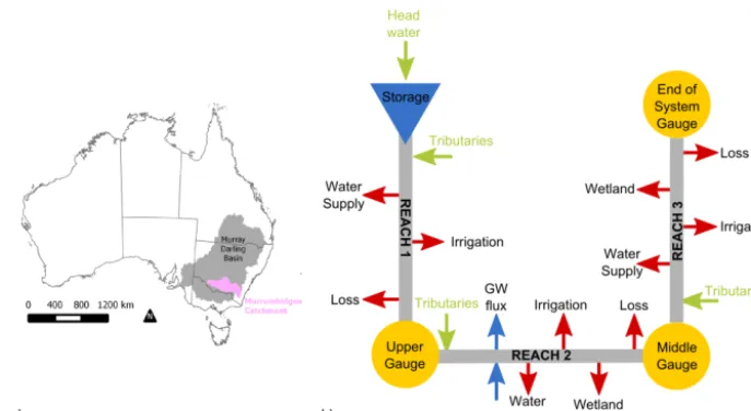
Figure 1. (a) Map showing the extent (indicated by pink shading) of the idealized river system model within the Murray–Darling Basin and (b) schematic structure of the river management model.
This implies that the methodology can be applied with ran-dom sampling, quasi-ranran-dom sampling (e.g. Latin Hyper-cube Sampling or Sobol’ sequences) or Markov chain Monte Carlo simulation.
The resulting data set is partitioned intoMclassesCmwith
m=1, . . . , M. For each classCm, the density function can be approximated with a kernel smoothing function with kernel
K(.)and bandwidthα(Devroye and Gyorfi, 1985):
ˆ
fY(y)= 1
n
n X
i=1 1
αK
y−y i
α
ˆ
fY|Cm(y)= 1
nm nm X
i:xi∈Cm 1
αm
K
y−y i
αm
, (3)
wherenmis the number of samples in classCmandαmthe corresponding bandwidth for the kernel smoothing function. The next step is to approximate the L1-norm between the two distributions for each class. Using a predefined number of quadrature points{ ˜yj, j=1, . . ., l}, the separation can be computed as
sm,j= ˆfY(y˜j)− ˆfY|Cm(y˜j)
ˆ
Sm= 1 2
l−1 X
j=1
|sm,j+1| + |sm,j|
˜
yj+1− ˜yj
. (4)
The sensitivity indexδcan then be approximated by
ˆ
δ= 1
2n
M X
m=1
nmSˆm. (5)
To avoid bias in the sensitivity index and to assess the ro-bustness of the sensitivity index estimate, it is recommended to perform a bootstrap of the sensitivity index (Efron, 1977)
and to adjustδˆwith the mean of the bootstrapδ¯∗:
ˆˆ
δ=2δˆ− ¯δ∗. (6)
ˆˆ
δ provides the sensitivity index of the main effect of a variable. Plischke et al. (2013) however does not provide a method to explore second-order effects, i.e. the interaction between two variables. To estimate second-order effects be-tween variablesX1andX2, the samples are subdivided into
ngroups of equal intervals forX1. The sensitivity indexδˆfor
X2,δˆX2, is computed for each interval. If there is no interac-tion effect betweenX1andX2, thenδˆX2 will not vary with the level ofX1. To quantify this, the variance ofδˆX2is com-puted over allnlevels ofX1. Small variances indicate small interaction effects and vice versa.
3 Model description and setup
The case study is a hypothetical river system model (Fig. 1), based on a simplified version of the Murrumbidgee River model in New South Wales, Australia (Dutta et al., 2012; Podger et al., 2014). Using the full version of the Mur-rumbidgee River model was not warranted, not only because of the complexity of the system and the management rules, but, more importantly, because of legal issues with regard to model licensing and confidentiality. The idealized, hypo-thetical model retains most of the relevant complexity prac-titioners encounter when creating water allocation models, which is more than sufficient to illustrate the sensitivity anal-ysis methodology.
[image:3.612.127.471.64.252.2]3780 L. J. M. Peeters et al.: Robust global sensitivity analysis of a river management model
Table 1. Output variables of the Source river system model.
Name Description Units
UpperFlow Flow rate at the gauge at the end of the first reach m3s−1 MiddleFlow Flow rate at the gauge at the end of the middle reach m3s−1 EndFlow Flow rate at the gauge at the end of the final reach m3s−1 $AlgalBloom Monetary value generated by recreation as function of the
risk of algal blooms
106AUD
$Stor Monetary value generated by recreation on storages 106AUD $TotalAg Monetary value generated by irrigated agriculture 106AUD Hydropower Electricity generated from the storage reservoir kWh GenSec Percentage of time general security licences receive their
full entitlement
%
from the system for town water supply and irrigation and wa-ter is received from unregulated rain-fed tributaries. From the Upper Gauge at the end of reach 1, water is routed through reach 2. In this reach, interaction with groundwater is taken into account by an exchange flux. As in reach 1, water is received from unregulated, rain-fed tributaries and water is taken out for irrigation and town water supply. In addition to these offtake, water is diverted into an off-river wetland system. Reach 3 starts at the middle gauge and is similar to reach 2. It also has offtake for town water supply, irrigation and off-river wetlands and receives inflow from rainfed trib-utaries. Groundwater–surface water interaction is not taken into account in this reach. Each reach has a term represent-ing unaccounted losses. The loss relationships are taken from the more complex model. The total travel time from headwa-ter to end-of-system is 18 days (3 days for reach 1, 6 days for reach 2 and 9 days for reach 3). These values, together with the other parameters influencing routing of water are also taken and aggregated from the more complex model.
Daily time series of rainfall and evaporation from 1895 to 2006 are obtained from SILO (http://www.longpaddock. qld.gov.au/silo/) for sites representative of each of the three reaches. These time series are used to simulate inflow from tributaries and compute irrigation demand. Inflow into the main storage in the model is taken from daily gauged data from 1895 to 2006.
The town water demands are based on a fixed annual pat-tern (8.8, 3.0 and 1.2×10⁶m3year−1for reaches 1, 2 and 3 respectively). Irrigation demands are based on a reach-based aggregation of irrigation use as well as rationalizing of crop types. There are environmental demands for the wetlands in reach 2 and 3, which are designed to establish and maintain favourable habitat conditions for indigenous fauna and flora (Janssen, 2012).
Two aspects of water management are considered: 347 m3s−1order constraint on storage releases, i.e. the max-imum flow that can be requested by water users in the system of the storage, and an annual allocation system. The alloca-tion system comprises high and general security order debit
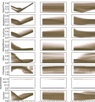
Figure 2. Scatter plots ofMˆ, the difference between kernel density estimates for each simulation and the kernel density estimate of the reference simulation for all forcing data and model output variables for the eWater Source hypothetical river management model.
Figure 3. Sensitivity indices,δˆˆ, for all forcing data and model out-put variables for the eWater Source hypothetical river management model.
4 Results
In the sensitivity analysis, the three main forcing variables are considered: the system inflow (Inflow), the precipitation (Rain) and the potential evapotranspiration (PET). The latter two affect the inflow into the reaches and the irrigation de-mand. Inspired by the work of Leblanc et al. (2012), the forc-ing variables are changed through a multiplier to the corre-sponding input time series with the range of the multiplier for each variable between 0.5 and 1.5. This range encompasses both historical variation in hydrological input and output, as well as the expected change under various climate change models and scenarios. While elaborate schemes are available to perturb hydrological time series, this is not warranted in this study as the focus is on metrics that integrate the entire flow time series. As such, the emphasis of this research is on changes in total flow in or out of the model, rather than in changes of the timing of flow.
[image:5.612.49.291.472.607.2]3782 L. J. M. Peeters et al.: Robust global sensitivity analysis of a river management model
Figure 4. Scatter plots of interaction of the driving forces. The
in-tensity of the colour scale is proportional to the model outcome value, where dark red indicates high values and light red indicates low values.
calculated (Pickett et al., 2013). Table 1 lists the names of the output series and a short description.
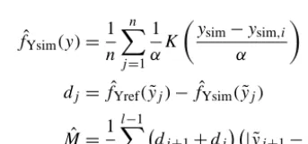
Each of the output variables in Table 1 is a daily time se-ries. The metric for the sensitivity for different forcing data (Mˆ) is the difference between the kernel density estimate of the daily times series of a randomly selected reference simu-lation (fˆYref(y)) and the kernel density estimate of the daily time series for the changed forcing data (fˆYsim(y)):
ˆ
fYref(y)= 1
n
n X
j=1 1
αK
yref−yref,i
α
[image:6.612.311.550.67.300.2]
Figure 5. Sensitivity indexδˆof the effect of Rain (blue) and PET (red) on $Stor for 100 equal intervals of Inflow.
ˆ
fYsim(y)= 1
n
n X
j=1 1
αK
y
sim−ysim,i
α
dj= ˆfYref(y˜j)− ˆfYsim(y˜j)
ˆ
M=1
2 l−1 X
j=1
dj+1+dj | ˜yj+1− ˜yj| (7)
The choice of this metric is motivated by the fact that, since the case study is an idealized, hypothetical model, it is not possible to directly compare the results with observations. In addition to this, and more importantly, the variety of model outcomes examined in this study are more than likely to be affected by different aspects of the hydrograph. Simi-lar to choosing an objective function in traditional calibra-tion or a likelihood funccalibra-tion in uncertainty analysis, such metric needs to be tailored to be able to capture the rele-vant aspects of the hydrograph. Choosing an ill-suited met-ric can have huge consequences for the sensitivity analysis, calibration or uncertainty analysis, as pointed out in Monta-nari and Koutsoyiannis (2012) and Nearing (2014). The met-ric presented in Eq. (7) is designed to provide an as gen-eral and robust as possible measure of the difference be-tween two time series as not to bias the interpretation of the sensitivity analysis.
4.1 Main effects
[image:6.612.307.479.355.435.2]Figure 6. Var(δˆX1−X2)for all combinations of driving forces for all model outcomes. High values indicate potential interaction betweenX1 andX2. The values for Hydropower are omitted in order not to distort the visualization.
a strong response is noticeable for variations in this driving variable for all output variables with the exception of Hy-droPower. The effects of “Rain” and “PET” are less pro-nounced. A very striking feature are the many nonlineari-ties in the response surface of the hypothetical model. This is mostly due to a number of threshold values used in the man-agement rules of the river manman-agement system. For instance, generation of hydro-power is only possible when the storage level in the dam exceeds a predefined threshold related to the height of the water intake point for the turbines.
Figure 3 shows a barplot of the sensitivity indices δˆˆfor all main effects. These indices confirm the dominant influ-ence of Inflow on most output variables. They provide a rel-ative ranking of the influence of the input variable Inflow on the various output variables. MiddleFlow, EndFlow and GenSec respond to a similar degree to changes in Inflow and the same is true for the output variables related to monetary value ($AlgalBloom, $Stor and $TotalAg). HydroPower is least influenced by Inflow, which, from Fig. 2, is clearly re-lated to the threshold-induced nonlinear behaviour.
The methodology is also able to quantify the often small and nonlinear effects of the other forcing variables. This is especially noticeable for PET. There is a clear but highly non-linear effect of PET on $Stor, which is reflected in a higherδˆˆ. The output variable HydroPower has a bimodal distribution where the majority of simulations have anMˆ close to zero. Nevertheless, the global sensitivity method is able to distin-guish and quantify the subtle trends in the non-zero values for the different input variables.
4.2 Interaction effects
The previous section established the importance of Inflow as the main driving variable. It is however from both a manage-ment and modelling perspective interesting to have an under-standing of how the interaction between variables affects the model outcome.
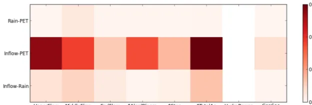
Figure 4 shows plots with the factor values on thex- and
y-axis, with a colour scale to visualizeMˆ for the three com-binations of interaction of the driving forces (Inflow-Rain, Inflow-PET and Rain-PET) for all eight model outcomes.
The first column shows that the effect of Inflow on most of the model outputs does not vary with the value of Rain. There is however a clear interaction between Inflow and PET for most of the model outputs; while the Inflow response is the dominant feature in the plots, the shape of this response de-pends on the value of PET. HydroPower is a noted exception as it displays very little structure in the scatter plots. This is because hydropower is generated by release of water from the reservoir in function of the demand and the water level in the reservoir. These management rules create a buffer to immediate impact from rainfall and inflow and also result in nonlinear, threshold related behaviour.
Very little structure is noticeable in the third column of Fig. 4, which shows the interaction between Rain and PET, reflecting the limited influence both driving forces have as a main effect.
To quantify the interaction effect for each interaction com-bination in Fig. 4, the variance of the δˆ of the variable on they-axis is computed for 100 equal intervals of the vari-able on thex-axis. By using Sobol’ sequences to generate the 100 000 samples of the parameter space, each equal in-terval of thex-axis variable has approximately 1000 samples to compute theδˆ.
Figure 5 illustrates this for the interaction effects of In-flow, Rain and PET on $Stor. The sensitivity index values for Rain are low and hardly vary for different levels of Inflow, which is an indication of very limited interaction between Rain and Inflow, as confirmed by the scatter plot (Fig. 4). Theδˆvalues for PET vary markedly with the level of Inflow. This sensitivity index reaches a minimum for Inflow values close to 1, while reaching peaks close to values of 0.75 and 1.1. This is reflected in the variance of theδˆvalues which is 4.5×10⁻⁴for the Inflow–Rain couple and 3.5×10⁻³for Inflow–PET. Figure 6 shows the variance of the sensitivity indices for all interaction pairs for all model outcomes. The values for Hydropower are much higher than for the other model outcomes due to the nonlinear behaviour. They were omitted from Fig. 6 as they distorted the visualization.
3784 L. J. M. Peeters et al.: Robust global sensitivity analysis of a river management model 5 Discussion
The sensitivity analysis of the hypothetical river management model highlights inflow as a crucial variable of the model and how this affects the economic, environmental and sociolog-ical functions of the river. This emphasizes the importance of an accurate characterization of the flow rates of upstream areas when modelling flow routing in regulated systems com-parable to the case study, i.e. the regulated river systems of the Murray–Darling Basin in Australia. An accurate charac-terization of flow rates not only entails maintaining a dense river gauge network, it also means adequately describing the measurement uncertainty in the flow rates, not in the least the uncertainty introduced by the rating curve that describes the stage–discharge relationship (Tomkins, 2012). The work of Hughes et al. (2014) illustrates this as they identify the in-flow from ungauged catchment as crucial in the calibration of river management models.
Direct precipitation in the storage, wetlands and irri-gation areas has a very minor influence on the model outcomes. This is mostly due to the small volume of rainfall (0.633 km3yr−1) compared to the inflow volume (4.4 km3yr−1) and the correlation between the inflow vol-ume and rainfall. Any effect of rainfall will therefore be dwarfed by the effect of inflow to the system. The interac-tion effect of Inflow and PET is mostly due to the feedback mechanism as irrigation requirements increase with increas-ing potential evapotranspiration.
Such parameter interaction is well known in other areas of hydrological modelling, such as in rainfall–runoff mod-elling (Gallagher and Doherty, 2007; Zhang et al., 2013; Peeters et al., 2013) and in groundwater modelling (Doherty and Hunt, 2009), although it has not received much atten-tion in river system modelling. Letcher et al. (2007) discuss the importance of interacting effects in water allocation mod-els, without however providing a rigorous quantitative frame-work to evaluate the effects.
The sensitivity analysis in this study was limited to mul-tiplying factors on three driving forces. It would be very in-sightful to include other model parameters in the sensitivity analysis, especially those controlling storage volumes and ir-rigation requirements. Along the same lines, including the parameters of the management rules, e.g. rules on alloca-tions, in the sensitivity analysis can yield additional under-standing of the operational management of the river system, as shown by Micevski et al. (2011).
6 Conclusions
The density-based sensitivity analysis of Plischke et al. (2013) has been applied to a river management model rep-resenting an idealized regulated river system representative of the southern Murray–Darling Basin in Australia to
iden-tify the main and interaction effects of three driving forces on several hydrological and socio-economic model outcomes.
The extended sensitivity analysis method presented in this paper provides a quantitative measure of sensitivity of the main and interaction effects and, through a combination with qualitative visual inspection of scatter plots, proved to be able to identify not only major effects but also subtle interactions, even in the presence of strong nonlinearities.
Due to the small dimensionality of the case study, it was possible to visualize all main effects and their interactions through scatter plots for all model outcomes. Although this will be challenging for higher-dimensional problems, the vi-sual inspection of scatter plots is an invaluable complement to the sensitivity indices.
Understanding the dynamics of river system models is of-ten not intuitive, especially in larger or basin-scale models (Johnston and Smakhtin, 2014). A robust and comprehen-sive sensitivity analysis is an invaluable step in model devel-opment to elucidate the often intricate interactions between driving forces, management rules and parameters. Increased understanding of the model will not only lead to improve-ments in calibration and prediction, it also has enormous po-tential in establishing the credibility and understanding of models.
Acknowledgements. The authors thank Russell Crosbie and Dave
Penton for their constructive comments.
Edited by: H. Cloke
References
Bark, R., Peeters, L., Lester, R., Pollino, C., Crossman, N., and Kan-dulu, J.: Understanding the sources of uncertainty to reduce the risks of undesirable outcomes in large-scale freshwater ecosys-tem restoration projects: An example from the Murray-Darling Basin, Australia, Environ. Sci. Pol., 33, 97–108, 2013.
Borgonovo, E.: A new uncertainty importance measure, Reliability Eng. Syst. Safety, 92, 771–784, 2007.
Borgonovo, E., Castaings, W., and Tarantola, S.: Moment Inde-pendent Importance Measures: New Results and Analytical Test Cases, Risk Anal., 31, 404–428, 2011.
Campolongo, F., Cariboni, J., and Saltelli, A.: An effective screen-ing design for sensitivity analysis of large models, Environ. Mod-ell. Softw., 22, 1509–1518, 2007.
Castaings, W., Dartus, D., Le Dimet, F.-X., and Saulnier, G.-M.: Sensitivity analysis and parameter estimation for distributed hy-drological modeling: potential of variational methods, Hydrol. Earth Syst. Sci., 13, 503–517, doi:10.5194/hess-13-503-2009, 2009.
Crase, L. and Gillespie, R.: The impact of water quality and water level on the recreation values of Lake Hume, Aust. J. Environ. Manage., 15, 21–29, 2008.
Doherty, J. and Hunt, R. J.: Two statistics for evaluating parame-ter identifiability and error reduction, J. Hydrol., 366, 119–127, 2009.
DRET: Destination visitor survey: strategic regional research report – New South Wales, Victoria and South Australia. Impact of the drought on tourism in the Murray River Region., Tech. rep., De-partment of Resources, Energy and Tourism, Tourism Research Australia, 57 pp., 2010.
Dutta, D., Hughes, J., Vaze, J., Kim, S., Yang, A., and Podger, G.: A daily river system model for the Murray-Darling Basin: devel-opment, testing and implementation, in: 34th Hydrology and Wa-ter Resources Symposium 2012, Sydney, 19–22 November 2012, 1057–1066, available at: http://www.hwrs2012.org.au/, 2012. Efron, B.: Bootstrap methods: another look at the jackknife, The
Annal. Stat., 7, 1–26, 1977.
Foglia, L., Hill, M. C., Mehl, S. W., and Burlando, P.: Sensitiv-ity analysis, calibration, and testing of a distributed hydrological model using error-based weighting and one objective function, Water Resour. Res., 45, W06427, doi:10.1029/2008WR007255, 2009.
Gallagher, M. R. and Doherty, J.: Parameter interdependence and uncertainty induced by lumping in a hydrologic model, Water Resour. Res., 43, W05421, doi:10.1029/2006WR005347, 2007. Gupta, H. V., Clark, M. P., Vrugt, J. A., Abramowitz,
G., and Ye, M.: Towards a comprehensive assessment of model structural adequacy, Water Resour. Res., 48, W08301, doi:10.1029/2011WR011044, 2012.
Hill, M. C. and Tiedeman, C. R.: Effective groundwater model cal-ibration, Wiley, 2007.
Hughes, J., Dutta, D., Vaze, J., Kim, S., and Podger, G.: An auto-mated multi-step calibration procedure for a river system model, Environ. Modell. Softw., 51, 173–183, 2014.
Janssen, V.: Indirect Tracking of Drop Bears Us-ing GNSS Technology, Aust. Geogr., 43, 445–452, doi:10.1080/00049182.2012.731307, 2012.
Johnston, R. and Smakhtin, V.: Hydrological Modeling of Large river Basins: How Much is Enough?, Water Resour. Manage., 28, 1–36, doi:10.1007/s11269-014-0637-8, 2014.
Leblanc, M., Tweed, S., Van Dijk, A., and Timbal, B.: A review of historic and future hydrological changes in the Murray-Darling Basin, Global Planet. Change, 80–81, 226–246, 2012.
Letcher, R. A., Croke, B. F. W., and Jakeman, A. J.: Integrated as-sessment modelling for water resource allocation and manage-ment: A generalised conceptual framework, Environ. Modell. Softw., 22, 733–742, 2007.
Micevski, T., Lerat, J., Kavetski, D., Thyer, M., and Kuczera, G.: Exploring the utility of multi-response calibration in river system modelling, 19th International Congress On Modelling and Sim-ulation (modsim2011), 12–16 December 2011, Perth, Australia, 3889–3895, 2011.
Montanari, A. and Koutsoyiannis, D.: A blueprint for process-based modeling of uncertain hydrological systems, Water Resour. Res., 48, W09555, doi:10.1029/2011WR011412, 2012.
Morrison, M. and Hatton MacDonald, D.: Economic valuation of environmental benefits in the Murray-Darling Basin, Tech. rep., A report to the Murray Darling Basin Authority, 2010.
Nearing, G.: Comment on “A blueprint for process-based modeling of uncertain hydrological systems” by
Monta-nari and Koutsoyiannis, Water Resour. Res., 50, 6260–6263, doi:10.1002/2013WR014812, 2014.
Nossent, J., Elsen, P., and Bauwens, W.: Sobol’ sensitivity analysis of a complex environmental model, Environ. Modell. Softw., 26, 1515–1525, 2011.
Patt, A.: Uncertainties in environmental modelling and conse-quences for policy making, chap. Communicating uncertainty to policy makers, pp. 231–251, NATO science for peace and secu-rity series – C: Environmental Secusecu-rity, Springer, available at: http://www.pik-potsdam.de/news/public-events/archiv/alter-net/ former-ss/2009/14.09.2009/patt/literature/bavaye-book.pdf, 2009.
Peeters, L., Lerat, J., and Rassam, D.: Improving parameter estima-tion in transient groundwater models through temporal differenc-ing, in: MODSIM 2011: Sustaining Our Future, 12–16 December 2011, Perth, Australia, p. 7, 2011.
Peeters, L., Crosbie, R., Doble, R., and Van Dijk, A.: Conceptual evaluation of continental land-surface model behaviour, Environ. Modell. Softw., 43, 49–59, 2013.
Pickett, T., Smith, T., Bulluss, B., Penton, D., Peeters, L., Podger, G., and Cuddy, S.: Approaches to distributed execution of hydro-logic models: methods for ensemble Monte Carlo risk modelling with and without workflows, in: MODSIM 2013 20th Interna-tional Congress on Modelling and Simulation, 1–6 December 2013, Adelaide, Australia, p. 7, 2013.
Plischke, E., Borgonovo, E., and Smith, C. L.: Global sensitivity measures from given data, Eur. J. Operational Res., 226, 536– 550, 2013.
Podger, G., Cuddy, S., Peeters, L., Smith, T., Bark, R., and Black, D.: Risk management frameworks: supporting the next genera-tion of Murray-Darling Basin water sharing plans, in: Evolving Water Resources Systems: Understanding, Predicting and Man-aging Water-Society Interactions, Proceedings of ICWRS2014, Bologna, Italy, June 2014 (IAHS Publ. 364, 2014, 452–457), 364, 452–457, 2014.
Saltelli, A. and Annoni, P.: How to avoid a perfunctory sensitivity analysis, Environ. Modell. Softw., 25, 1508–1517, 2010. Saltelli, A., Ratto, M., Andres, T., Campolongo, F., Cariboni,
J., Gatelli, D., Saisana, M., and Tarantola, S.: Global Sen-sitivity Analysis. The Primer, John Wiley & Sons, Ltd, doi:10.1002/9780470725184, 2008.
Sobol, I.: Uniformly distributed sequences with an additional uni-form property, USSR Comput. Mathem. Mathem. Phys., 16, 236–242, 1976.
Tomkins, K. M.: Uncertainty in streamflow rating curves: meth-ods, controls and consequences, Hydrol. Process., 28, 464–481, doi:10.1002/hyp.9567, 2012.
Wagener, T. and Kollat, J.: Numerical and visual evaluation of hydrological and environmental models using the Monte Carlo analysis toolbox, Environ. Modell. Softw., 22, 1021–1033, 2007. Welsh, W. D., Vaze, J., Dutta, D., Rassam, D., Rahman, J. M., Jolly, I. D., Wallbrink, P., Podger, G. M., Bethune, M., Hardy, M. J., Teng, J., and Lerat, J.: An integrated modelling framework for regulated river systems, Environ. Modell. Softw., 39, 81–102, 2013.