www.hydrol-earth-syst-sci.net/19/17/2015/ doi:10.5194/hess-19-17-2015
© Author(s) 2015. CC Attribution 3.0 License.
Multi-scale analysis of bias correction of soil moisture
C.-H. Su and D. Ryu
Department of Infrastructure Engineering, University of Melbourne, 3010 Victoria, Australia Correspondence to: C.-H. Su ([email protected])
Received: 1 July 2014 – Published in Hydrol. Earth Syst. Sci. Discuss.: 29 July 2014 Revised: 2 December 2014 – Accepted: 4 December 2014 – Published: 6 January 2015
Abstract. Remote sensing, in situ networks and models are now providing unprecedented information for environmen-tal monitoring. To conjunctively use multi-source data nomi-nally representing an identical variable, one must resolve bi-ases existing between these disparate sources, and the char-acteristics of the biases can be non-trivial due to spatio-temporal variability of the target variable, inter-sensor differ-ences with variable measurement supports. One such exam-ple is of soil moisture (SM) monitoring. Triexam-ple collocation (TC) based bias correction is a powerful statistical method that is increasingly being used to address this issue, but is only applicable to the linear regime, whereas the non-linear method of statistical moment matching is susceptible to unin-tended biases originating from measurement error. Since dif-ferent physical processes that influence SM dynamics may be distinguishable by their characteristic spatio-temporal scales, we propose a multi-timescale linear bias model in the frame-work of a wavelet-based multi-resolution analysis (MRA). The joint MRA-TC analysis was applied to demonstrate scale-dependent biases between in situ, remotely sensed and modelled SM, the influence of various prospective bias cor-rection schemes on these biases, and lastly to enable multi-scale bias correction and data-adaptive, non-linear de-noising via wavelet thresholding.
1 Introduction
Global environmental monitoring requires geophysical mea-surements from a variety of sources and sensors to close the information gap. However, different direct and remote sens-ing, and model simulation can yield different estimates due to different measurement supports and errors. Soil moisture (SM) is one such variable that has garnered increasing in-terest due to its influences on atmospheric, hydrologic,
geo-morphic and ecological processes (Rodriguez-Iturbe, 2000; GLACE Team et al., 2004; Legates et al., 2011). It also rep-resents an archetype of the aforementioned problem, where in situ networks, remote sensing and models jointly provide extensive SM information.
In situ networks usually provide point-scale measure-ments; satellite retrieval of shallow SM at a mesoscale foot-print of 10–50 km must resort to a homogeneity or dominant-feature assumption, whereas modelled SM depends on the simplified model parameterization, and the quality, resolu-tion and availability of forcing data. Subsequently, the spatial (lateral and vertical) variability of SM can lead to systemat-ically different measurements regarded as biases. Descrip-tive or predicDescrip-tive spatial SM statistics can be used to relate point-scale to mesoscale estimates (Western et al., 2002), but in situ data are often limited in describing the spatial het-erogeneity of SM. However, without bias correction, it is not possible to conduct meaningful comparisons between in situ, satellite-retrieved and modelled SM for validation (Re-ichle et al., 2004) and optimal data assimilation (Yilmaz and Crow, 2013). Standard bias correction methods are now in-creasingly being applied to SM assimilation in land models (Reichle et al., 2007; Kumar et al., 2012; Draper et al., 2012), numerical weather prediction (Drusch et al., 2005; Scipal et al., 2008a) and hydrologic models (Brocca et al., 2012). Reichle and Koster (2004) proposed matching statistical mo-ments of the data, while linear methods based on simple re-gression and matching dynamic ranges have also been con-sidered (e.g. Su et al., 2013a). But these methods can induce artificial biases in the signal component of the corrected data as the error statistics were ignored; this also suggests a con-nection that the issue of bias correction is inseparable from that of error characterisation (Su et al., 2014a).
2014a), is increasingly being used to address these issues in oceanography (Caires and Sterl, 2003; Janssen et al., 2007) and hydrometeorology (Scipal et al., 2008b; Roebeling et al., 2013). In particular, it was used to estimate spatial point-to-footprint sampling errors (Miralles et al., 2011; Gruber et al., 2013), and correct biases in SM (Yilmaz and Crow, 2013). Based on an affine signal model and additive orthogonal er-ror model, it assumes that representativity differences are manifested as additive and multiplicative biases. But these assumptions may have limited validity, as the temporal be-haviour of SM may vary across different spatial scales, driven by a continuum of localised and mesoscale influences (e.g. Entin et al., 2000; Mittelbach and Seneviratne, 2012). Specif-ically, the coupling of SM with precipitation and evapora-tive losses (controlled by temperature, humidity, wind speed) varies across spatial scales. This can be more pronounced at places where surface hydrological features (e.g. topog-raphy, infiltration rate and storage capacity) are highly het-erogeneous. Thus, the biases are likely to be non-systematic across short and long timescales on different spatial scales and errors are non-white, undermining the utility of the affine model. One possible remedy is to apply bias correction, ei-ther TC or statistical-moment matching, only to anomaly time series (Miralles et al., 2011; Liu et al., 2012; Su et al., 2014a), but it remains unclear how these methods affect the signal and noise components in the corrected data. Alterna-tively a moving time window can be used to examine the time-varying statistics of time series (Loew and Schlenz , 2011; Zwieback et al., 2013; Su et al., 2014a).
Given the possible (time)scale dependency in biases and errors, we propose an extension to TC analyses to in-clude wavelet-based multi-resolution analysis (MRA) (Mal-lat, 1989) as a framework to (1) provide a fuller description of the temporal scale-by-scale relationships between coinci-dent data sets; (2) study the influence of various prospec-tive bias correction schemes; and (3) achieve multi-scale bias correction. To avoid excessive changes in the noise charac-teristics upon correction, TC can be further combined with the wavelet thresholding (Donoho and Johnstone, 1994) to (4) achieve non-linear, data-adaptive de-noising, with con-trast to existing linear schemes (Su et al., 2013b). The tech-niques were applied to SM data from an in situ probe, satel-lite radiometry and land-surface model, but the proposed methods are generally enough to be applied to other geophys-ical variables.
The paper is organised as follows. Section 2 presents the study area over Australia and the SM data sets used in our pilot studies. Section 3 explains the theoretics behind MRA and applies it to SM, following by examination of scale-by-scale statistics in Sect. 4. Section 5 presents a new joint MRA-TC analysis framework, which is then applied to ex-amine the influence of different bias correction schemes in Sect. 6. Importantly, both Sects. 4 and 6, using wavelet cor-relation, wavelet variance and scale-level TC analyses, pro-vide epro-vidence to support the need to extend traditional bulk
and anomaly based analyses. Section 7 demonstrates the use of wavelet thresholding to de-noise satellite SM. Section 8 offers our concluding remarks.
2 Study areas and data sets
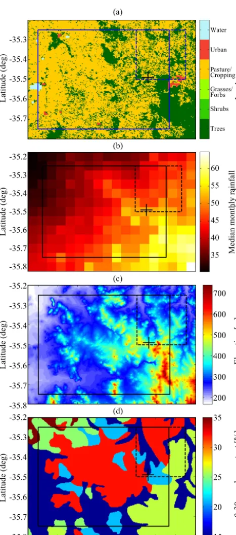
We consider in situ, satellite-retrieved and modelled SM over Australia. For an in-depth study, we consider point-scale and pixel-point-scale SM estimates at K1 monitoring site (147.56◦ longitude,−35.49◦ latitude) situated at Kyeamba Creek catchment, southeastern Australia (Smith et al., 2012; Su et al., 2013a). The in situ SM (INS as shorthand) was sampled at 30 min intervals, 0–8 cm depth using a time-domain interferometer-based Campbell Scientific 615 probe during November 2001–April 2011. The region experiences a temperate (Cfb) climate characterised by seasonally uni-form rainfall but variable evapotranspiration forcing, so that SM varies between dry in summer (December–February) to wet in winter (June–August). The creek is located on gentle slopes with rain-fed cropping and pasture, and the soil varies from sandy to loam. Figure 1 illustrates the land cover, ele-vation, monthly rainfall accumulation (from 2002 to 2011), and clay content over the region.
The satellite SM was retrieved by AMSR-E (Advanced Microwave Scanning Radiometer for Earth Observing Sys-tem; AMS) of the AQUA satellite. The retrieval is based on an inversion of the forward radiative transfer model of a vegetation-masked soil surface, relating observed brightness temperature to soil dielectric constant estimates. A dielectric mixing model is then used to related the dielectric constant to volumetric SM. The combined C/X-band 1/4◦×1/4◦
grid-ded, half-daily (∼1.30 a.m./p.m. LT – local time) version 5 product (July 2002–October 2011) is based on the Land Pa-rameter Retrieval Model (Owe et al., 2008). C-band (X-band) has a shallow sampling depth of ∼1–2 cm (∼5 mm), al-though it is mostly C-band data over Australia due to rela-tively small radio frequency interference. Given the 1–2 day revisit times of the satellite, there is a significant number of missing values in the AMS data. However, we found that (not shown) over 99 % (95 %) of the gaps over Australia are ≤1.5 day (≤1 day) long. For use in wavelet analysis (Sect. 4), a one-dimensional (1-D in time) interpolation al-gorithm (Garcia, 2010) based on discrete cosine transform (Wang et al., 2012) was applied to infill gaps of lengths ≤5 days in AMSR-E. Other interpolation methods were tri-alled; e.g. linear interpolated AMSR-E shows great similari-ties to the DCT interpolated data, while cubic spline interpo-lation leads to spurious peaks.
sens-Figure 1. Spatial variability of land surface and rainfall over
Kyeamba Creek. The cross denotes the location of the K1 moni-toring station, and the dashed (solid) box is the pixel area of AMS (MER).
ing of precipitation and radiation (Rienecker et al., 2011). The MERRA land-only fields were post-processed by reinte-grating a revised Catchment model with more realistic pre-cipitation forcing to produce the MERRA-Land (MER as shorthand) data set (Reichle et al., 2011). The resultant SM field corresponds to the hourly averages of the uppermost layer (0–2 cm) and is gridded on a 2/3◦×1/2◦grid.
The three data are co-located spatially via nearest neigh-bour and temporally at around the satellite overpass times of 1.30 a.m./p.m. LT. Their time series are plotted in blue in the first panels of Fig. 2. While co-located, the three methods ob-served SM dynamics over different locations and areas of the catchment (Fig. 1), due to differences in their pixel resolu-tions and alignments.
Continental-scale AMS and MER data over Australia are also considered. The continent has great variability in cli-matic and land surface characteristics. Most of the northern regions experience a tropical savannah (Aw) Köppen–Geiger climate as classified by Peel et al. (2007), central Australia is largely arid desert (BWh), and eastern mountainous ar-eas have a temperate climate with no dry sar-easons (Cf). The southwestern regions similarly have a temperate climate, but with dry summers (Cs). These temperate regions have higher vegetation compared to the tropical north with moderate veg-etation cover.
3 Multi-scale decomposition of soil moisture
The observed Kyeamba SM (denoted by blue curves p in Fig. 2) exhibits a long-term cycle of wet and dry years due to the El Niño–Southern Oscillation and seasonal and diur-nal cycles originating from the fluctuations in vegetation and solar radiation, and experiences transient decay from various loss mechanisms, and abrupt increase from individual rain-fall events. Their influences on observed SM can vary with the measurement methods. To unravel these differences, we turn to wavelets as the analysing kernels to study variability on individual broad-to-fine timescales. The scale under in-vestigation is temporal for the rest of the paper, unless stated otherwise.
The 1-D orthogonal discrete wavelet transform (DWT) en-ables MRA of a time seriesp(t )of dyadic lengthN=2J and
a regular sampling interval1t by providing the mechanism to go from one resolution to another via a recursive function
pj(a−)1(t )=pj(a)(t )+pj(t ), (1)
with an expectation value E(p(ja))=E(p)=p(Ja)(t )=µp
and E(pj)=0, where the superscript (a) labels
[image:3.612.52.286.98.626.2]02 03 04 05 06 07 08 09 10 11 12 p8 p7 p6 p5 p4 p3 p2 p1
p(t)
(a) INS
De
ta
il
pj
02 03 04 05 06 07 08 09 10 11 12
p(a) 8
p(a) 7
p(a) 6
p(a) 5
p(a) 4
p(a) 3
p(a) 2
p(a) 1
p(t)
Timet(year)
A pp ro xim at io n p ( a ) j
02 03 04 05 06 07 08 09 10 11 12
p8 p7 p6 p5 p4 p3 p2 p1
p(t)
(b) AMS
02 03 04 05 06 07 08 09 10 11 12
p(a) 8
p(a) 7
p(a) 6
p(a) 5
p(a) 4
p(a) 3
p(a) 2
p(a) 1
p(t)
Timet(year)
02 03 04 05 06 07 08 09 10 11 12
p8 p7 p6 p5 p4 p3 p2 p1
p(t)
(c) MER
02 03 04 05 06 07 08 09 10 11 12
p(a) 8
p(a) 7
p(a) 6
p(a) 5
p(a) 4
p(a) 3
p(a) 2
p(a) 1
p(t)
Timet(year)
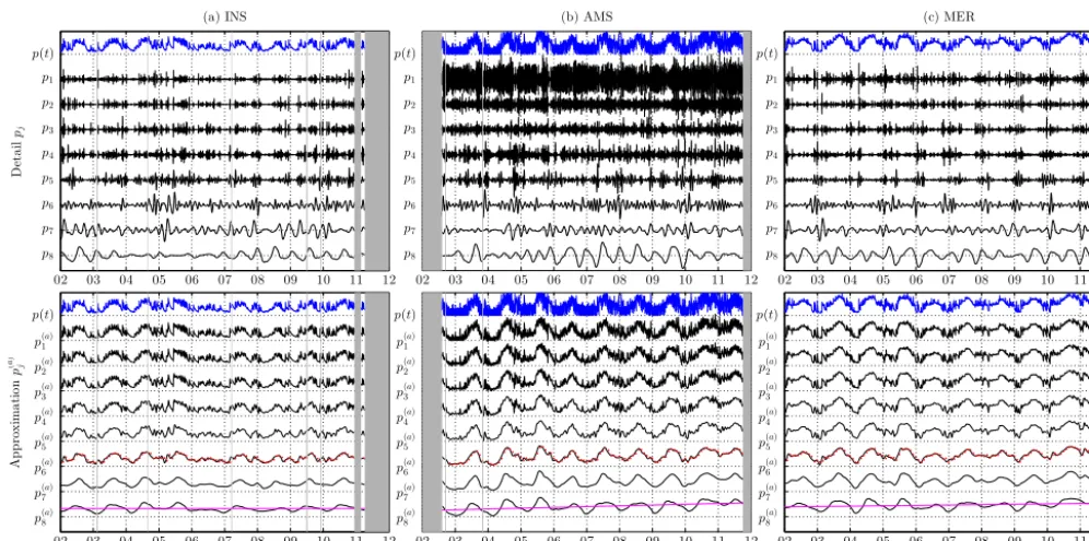
Figure 2. MRA of INS, AMS and MER SM at Kyeamba.pdenotes the original time series,pjthe detail time series, andpj(a)the
approxi-mation time series. Grey shadings are>5 day data gaps, red dots superimposed inp(6a)are monthly means ofp, and magenta lines are trend
lines fitted top8(a).
that at a higher resolution pj(a−)1 by adding some fine-scale detail denoted by pj. The end of the recursion chain leads
to reconstruction of the original time series with the equality
p(0a)(t )=p(t ), and a multi-resolution decomposition ofpas
p(t )=pj(a)
0 (t )+
j0
X
j=1
pj(t ) (2)
=
nj0
X
k=1 pj(a)
0kφj k(t )+
j0
X
j=1 nj
X
k=1
pj kψj k(t ) (3)
under j0 levels of decomposition. Loosely speaking, for
a half-daily time series, the detail time series pj for
j=1, 2, 3, . . . corresponds to (fine-scale) dynamics observed on 1 day (1 d), 2 d, 4 d, etc., timescales, while the approxima-tion time seriesp(ja)forj=1, 2, 3, . . . contains (broad-scale) dynamics on scales longer than 1 d, 2 d, 4 d, etc.
In Eq. (3), each of these components is further decom-posed into a linear summation ofnj=N/2j number of ba-sis functionsφj k andψj kwith scale of variability 2j1tand
temporal locationk2j1t. The weighting or wavelet coeffi-cients, determined via DWT ofp, measure the similarity be-tweenpand the bases via the inner productspj k(a)≡ hp, φj ki
andpj k≡ hp, ψj ki. Hence the coefficients indicate changes
on a particular scale and location, and enable the above scale-by-scale decomposition. Note that the bases are de-fined inL2(R)space and satisfy orthonormality conditions
prescribed byhφj k, φj0k0i =δj j0δkk0,hψj k, ψj0k0i =δj j0δkk0, hφj k, ψj0k0i =0, whereδis the Kronecker delta function. For detailed expositions of the mathematical theory of wavelets and MRA, consult Daubechies (1992) and Mallat (1989).
The detail and approximated time series of Kyeamba’s SM are illustrated in subsequent panels of Fig. 2, analysed using the DaubechiesD(4) wavelet forj0=8. On the finest scales j=1–2 (1–2 d), the details show variability due to rainfall wetting, and over the next set of scalesj=2–5 (2–16 d) they describe transient moisture loss. The p(6a) (≥32 d) compo-nent accounts for several scales of fluctuations over seasonal, inter-annual, and long-term timescales. For comparison, the standard monthly average analyses of the original time se-riespare superimposed onp(6a)(red dots).
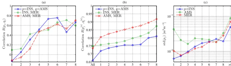
[image:4.612.47.545.64.311.2]1 2 3 4 5 6 7 8 0 0.2 0.4 0.6 0.8 1 Scalej C o rre la ti o n R ( pj ,qj ) (a)
p=INS,q=AMS INS, MER AMS, MER
All 1 2 3 4 5 6 7 8
0.65 0.7 0.75 0.8 0.85 0.9 0.95 1 Scalej C o rre la ti o n R ( p ( a ) j ,q ( a ) j ) (b)
p=INS,q=AMS INS, MER AMS, MER
1 2 3 4 5 6 7 8 >8 All
[image:5.612.98.495.67.181.2]10−2 10−1 Scalej st d ( pj )[ m 3m − 3] (c) p=INS AMS MER
Figure 3. Comparisons of correlationRand SD between INS, AMS and MER at scale levels. (a) compares the correlation between their detail time seriespj, and (b) compares between their approximation time seriespj(a). Scalej >8 corresponds top
(a)
8 , and “All” refers to
statistics of the original time series.
4 Multi-scale statistics
MRA enables direct comparisons between any two represen-tationsp= {X, Y}of a given variablef (e.g. SM) on vari-ous temporal scales independently, owing to the orthonormal properties of wavelet bases. It also offers an additional de-gree of freedom in temporal positions (using the indexk) to allow better representation of local variability. By subsetting the wavelet coefficients over certain range ofkvalues, non-stationary statistics can also be examined. However, in this work, we consider only variability acrossj and assume sta-tionarity on each scale. Pearson’s linear correlation R and variance analyses (see Appendix A) are performed on the Kyeamba’s INS, AMS and MER SM (as p in Eq. 2) de-tail (pj) and approximation (p(ja)) time series in Fig. 3. The strength of MRA is that since the detail time series pj on a given scale j does not contain variations on timescales greater thanj, the weak-sense stationarity conditions can be better met.
Before proceeding, we recall that weak R indicate the presence of noise and/or the presence of non-linear corre-lation between any pairs of the data, while differences in standard deviation can also indicate the presence of noise, but also an extraneous signal and/or multiplicative bias. Typ-ically one invokes a linearity assumption and assumes an affine relation between the signal components of the differ-ent data and an additive noise model (more later in Sect. 5), so that the differences between the data are attributed only to an overall additive bias E(X)−E(Y ), multiplicative bi-ases, and noise. While we adopt this simplistic viewpoint here, its limitations to properly account for variable lateral and vertical measurement supports should be noted. For in-stance, short-timescale SM dynamics show increasing atten-uation in amplitude, but are also delayed in time in deeper soil columns (e.g. Steelman et al., 2012). Additionally, SM is physically bounded between field capacity and residual con-tent and these thresholds can vary with soil texture, location and depths. These effects can give rise to temporal autocor-relation in errors and undermine the linearity assumption
be-tween coincident measures. Finally, the non-stationary char-acteristic of noise in satellite SM (Loew and Schlenz , 2011; Zwieback et al., 2013; Su et al., 2014a) due to e.g. dynamical land surface characteristics such as soil moisture (Su et al., 2014b), is not treated here.
With these considerations, we first examine the corre-lations between the three data. For the detail time se-ries (Fig. 3a), their correlations are lowest on the finest scales (R <0.2) but generally improves with scale (R >0.5), as noted previously. There is however no data pair that shows consistently higher R than other pairs: R(INSj,
AMSj) > R(INSj, MERj) on coarser scales j=4–6, 8,
whereasR(INSj, MERj) is highest on other scales.
Com-paring their approximation time series (Fig. 3b),Rbetween AMS and MER are higher than the other two pairs, ranging from (j=2) 0.8 to 0.92 (j=8), largely due to the strong cor-relation between their respectivep8andp(8a). In other words:
on one hand, AMS and MER both show skill in representing some aspects of the in situ SM temporal variability; on the other hand, stronger AMS-MER correlations on the coars-est (temporal) scales and their mesoscale spatial resolutions would indicate lesser representativeness of in situ measure-ment on these spatio-temporal scales.
Furthermore, we observe thatR(p(ja),qj(a)) reduces with decreasingj as more components are added to the recon-struction ofp(ja) andqj(a). The inclusion of noisy AMS1in
the makeup of AMS leads to a drop inR(INS, AMS) and
R(AMS, MER). Aside from including more noise in the approximation time series, adding components with differ-ent multiplicative biases (more later in Sect. 6) can also di-minish the correlations. The scale dependence of multiplica-tive biases and added noise can contribute to the contrasting results of applying TC to raw versus anomaly SM time se-ries in Draper et al. (2013). In particular, given the presence of noise inpj forj≥7, error analysis of the anomaly SM (i.e. inpj forj≤6) will under-estimate the total error in the
raw datap.
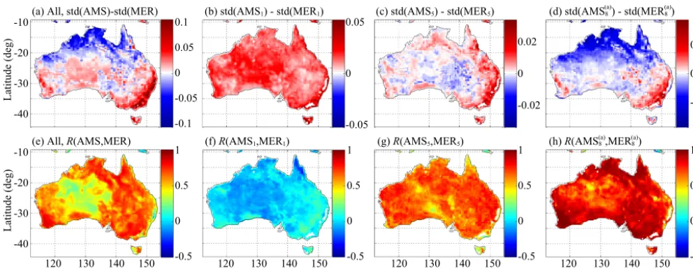
Figure 4. Difference in SD (in units of m3m−3) and correlationRbetween AMS and MER for (a, e) all and (rest) on selected timescales.
var(pj)≡std(pj)2. The three data show clear differences in
their standard deviation (SD) profile, both in the fine and coarse scales. As already noted, both noise and/or multiplica-tive biases are possible contributing factors such that noise can inflate the variance, while biases can cause suppression or inflation. Following the visual inspection of Fig. 2 and the noted weak correlations R(INSj, AMSj) and R(INSj,
MERj) at smallj, it can be argued that there is significant
noise in AMS (forj=1–3) and MER (j=1). This in turn leads to their larger SD cf. INS. On coarser scales where
R values are significantly higher, the differences in SD may be attributed more to multiplicative biases. For instance for theirp8andp8(a)components, AMS and MER shows larger
SD and thus positively biased relative to INS.
Figure 4 extends the variance and correlation analyses be-tween AMS and MER to the Australian continent using their coincident data from the period July 2002–October 2011. The spatial maps of SD differences (1SD) and correlations show significant variability in the statistics with timescales and spatial locations. On the finest scale j=1, the similar-ity between the difference map (Fig. 4a) and the TC-derived error map of AMSR-E (see Fig. 6a in Su et al., 2014a) in terms of spatial variability and the low AMS-MER correla-tions (Fig. 4f) support our observation that the detail time series AMS1 is noise dominated. Weak negative correlation
between AMS1and MER1can also be observed over arid
re-gions. By contrast, owing to the strong correlationR∼0.6– 0.9 (Fig. 4g and h) on the coarse scales, the causes of1SD (Fig. 4c and d) are related to biases. In particular, atj >8, the1SD map in Fig. 4d also suggests a possible association between biases and climatology or land cover characteristics, with negative biases dominating northern tropical (Aw) and semi-arid (BS) regions, and positive biases in temperate, veg-etated regions (Cs and Cf) over southeastern and
southwest-ern Australia. The visual comparisons between scale-level
1SD and bulk1SD enable stratification of the continent to central arid regions of higher noise identified inj=1 and 2 and temperate (tropical) regions, with a positive (negative) bias seen on coarser scales.
5 Joint MRA-TC analysis
In order to quantify observed differences between the data, we propose a scale-dependent linear model: a multi-scale (MS) model that distinguishes the signal components of the two dataX andY via an overall additive bias and a set of positive scaling coefficientsαp,j,α0p, and assumes an addi-tive and zero-mean independent but non-white noise model
p(t ). Focusing on the zero-mean signal and noise
compo-nents, the “structural relationship” model reads
p0(t )=α0pf0(t )+p0(t ), (4)
pj(t )=αp,jfj(t )+p,j(t ), (5)
for p0=p(ja)
0 −E(p) and f=f
0−E(f ), where the signal
MSD=(µX−µY)2+ J X
j h
αY,j−αX,j 2
var fj
+var X,j
+var Y,j
. (6)
The first term is the additive bias, and the summation con-sists of scale-specific multiplicative biases proportional to (αX,j−αY,j)2and noise contributions from each datum. The interpretation of the discrepancies betweenXandY can vary depending on the time period of the data and the analysis, and the adopted signal/noise model. By using the entire 9 year record of INS, AMS and MER data in MRA, the MS model does not observe a time-varying additive bias (e.g. from using the moving-window approach of Su et al., 2014a) or autocor-related errors (from using the lagged covariance in Zwieback et al., 2013). Rather, MRA and the MS model enable a de-scription of the systematic differences based wholly in terms of multiplicative biases at individual timescales, and the ran-dom differences in terms of additive noise. Specifically, this contrasts with the short time-window approach (e.g.≤32 d), where multiplicative biases existing on coarse scales (p6(a)) will manifest as both time-varying additive and multiplica-tive biases.
Importantly, the model allows for different scaling co-efficients between scales, i.e. αp,j6=αp,j0 for j6=j0, as a form of non-linearity with f. The equalityαp,j=α0p=αp
is therefore a special case of (bulk) linearity. As our focus of the above model is the multiplicative biases and noise, for convenience of notation, we remove the mean of theXandY
prior to MRA and bias correction. Furthermore, without the loss of generality, we chooseX as the reference henceforth and letαX,j,αX0 =1.
By using a third independently derived representation (Z) of f, TC enables estimation of the required scaling coeffi-cients and noise std(p,j) (Appendix B). As we will see later,
these estimates are needed for bias correction and de-noising. Within the operating assumptions of TC, TC estimates are unbiased and consistent; that is, the estimatedαY,jˆ =αY,j as the asymptotic limit. However, TC’s superiority is dependent on the availability of a strong instrument and a large sam-ple for statistical analyses (Zwieback et al., 2012; Su et al., 2014a). Standard linear estimators, namely ordinary least-square (OLS) regression and variance matching (VAR), can be considered as substitutes, although they are biased estima-tors ofαwhenX andY are both noisy (Yilmaz and Crow, 2013; Su et al., 2014a), e.g. OLS yieldsαˆY,j< αY,j. In
sum-mary, we propose that combining these estimators with MRA via the MS linear model enables investigation into the distri-bution of the multiplicative biases and additive noise overj, and their response to various bias correction schemes.
6 Multi-scale analysis of bias correction
Consider now the bias correction of Y to produce a cor-rected datumY∗that “matches”X. Different interpretations of a “match” and assumptions about signal and noise statis-tics lead to different bias correction schemes. To describe matching, there are different choices of optimality criterion. The first is based on matching the statistics of the signal-only component ofY∗to that ofX. This approach requires consistent estimation of slope parametersα’s and the resul-tant statistics ofXandY∗may differ due to different noise statistics. The second is based on the matching of the statis-tical moments betweenY∗ andX (e.g. VAR matching), al-though the statistics of their constitutive signal components may differ for the same reason. The third is based on the minimum-variance principle of minimizing the least-square difference betweenY∗ andX(i.e. the OLS estimation), but as already noted, the estimator becomes inconsistent when there are measurement errors inXandY.
Following our theoretical model in Sect. 5, we define our optimality criterion based on the first criterion of matching the first two moments of the signal components inX andY
so thatY∗is suitable for bias-free data assimilation. In partic-ular, Yilmaz and Crow (2013) have shown that residual mul-tiplicative biases due to a sub-optimal bias correction scheme will cause filter innovations to contain residual signal and sub-optimal filter performance. Thus, within the paradigm of the MS model, our goal of bias correction is to minimise the difference|αY∗,j −1|forαX,j=1, so that the multiplicative bias terms in Eq. (6) are eliminated.
– Bulk linear rescaling assumes bulk linearity betweenX
andY so that the correction equation is
Y∗= Y ˆ
αY
, (7)
whereαˆY is given by TC for our objective. When the
bulk linearity is satisfied, this approach ensures that the statistical properties (SD and higher moments) of the signal components in X and Y∗ are identical. Linear rescaling usingαYˆ values estimated by OLS and VAR matching have previously been considered by e.g. Su et al. (2013a); but due to error-in-variable biases, they can induce artificial biases in the signal component of
Y∗even if the bulk linearity condition is valid.
– Bulk cumulative distribution function (CDF) matching assumes non-linearity betweenXandY and transforms
Y∗so that (Reichle and Koster, 2004)
cdf Y∗=cdf(X), (8)
where cdf(◦) computes the CDF. This ensures that the mean, SD, and higher statistical moments ofXandY∗
not necessarily identical. In particular, when the relative signal and noise statistics in the two data are different, CDF matching leads to artificial biases between the sig-nal components inXandY∗. As with VAR matching of first two moments, the CDF counterpart is expected to contain extraneous contribution of the noise variances in the mapping of the second moment, as well as at higher moments (Su et al., 2014a). The issue can be exacer-bated by variable signal and noise statistics on different scales.
– Anomaly/seasonal (A/S) linear rescaling allows biases betweenXandY to be different on two scales of vari-ation. In practice, the useful information content in ob-servations is primarily based on their representation of anomalies, where observations are assumed in a partic-ular land surface model’s unique climatology (Koster et al., 2009). The correction is therefore limited to the anomalies, although other components (e.g. seasonal fluctuation and long-term trend) may be preserved to validate model prediction. Here the linear correction us-ing TC estimator is applied to match the characteristics of each component – anomaly (i=A) and seasonal (S) – separately, so that the correctedY has the form
Y∗=YS∗+YA∗, (9)
with Yi∗=Yi/αYˆ i for i∈ {S, A}. In one approach, pS
is computed using moving window averaging of multi-year data within a window size of 31 days centered on a given day of year (Miralles et al., 2011; Su et al., 2014a), so that inter-annual cycles and long-term trends are retained inpA. In an alternative approach (Albergel
et al., 2012), a sliding 31 day window is used such that
pA≈ 6
P
j=1
pjfor half-daily time series. In this work, the former, more conventional approach was taken. – A/S CDF matching applies CDF matching to anomaly
and seasonal components separately as per Eq. (9) but with cdf(Yi∗)=cdf(Xi). The application of CDF
match-ing to the anomaly component of soil moisture data was considered by Liu et al. (2012).
– Multi-scale (MS) rescaling is the direct consequence of the MS model where information inY is rescaled at in-dividual scales,
Y∗= Y 0
ˆ
αY0 + j0
X
j=1 Yj
ˆ
αY,j. (10)
In relation to Eq. (6), this approach obviously elimi-nates that the multiplicative terms in the summation. The bulk and A/S linear correction schemes can be con-sidered as special cases of MS rescaling where informa-tion from multiple scales are aggregated and corrected
jointly. Other aggregations of the information from dif-ferent subsets of scales are also possible, but they will similarly be conceived based on one’s understanding or assumptions of the underlying specific processes driv-ing SM dynamics. Investigations into suitable aggre-gations are beyond the scope of this work, hence we implemented the most elaborate decomposition. If joint linearity exists between two or more scales, theirαY,j
values will be similarly valued for use in Eq. (10). For illustrations, we correct the biases in AMS and MER SM with respect to INS SM at Kyeamba using the above five schemes. Using the above notations, AMS and MER are treated asY, the corrected AMS∗and MER∗asY∗, and INS asX. MRA-TC was applied to observe their consequences in Fig. 5. In the upper panel, estimatedαY,jˆ andαYˆ ∗,j val-ues provide diagnostics for detecting the presence of multi-plicative biases before and after application of the correction schemes. The lower panel plots the SD ofYjandYj∗and their
associated noisesY,jandY∗,j. The values of the scaling co-efficientsαY,j (before correction) andαY∗,j (after), and the noise std(Y,j) and std(Y∗,j) were estimated using TC. But where TC estimates could not be retrieved (forj=1–2) due to negative correlation amongst the data triplet (e.g. resulting from significant noise and weak instrument), OLS-derived (under) estimates serve as a guide for the above diagnostic purposes. Similarly, the total SD is a guide for noise SD in these cases.
Figure 5a shows the MRA of the biases and noise in the pre-corrected dataY. There is considerable variability inαY,jˆ across the scales, ranging from 0.5 to 1.8 for AMS, and from 0.5 to 1.4 for MER. In particular, theirαˆ0Y andαY,ˆ 8deviate
significantly from 1, and are responsible for the larger SD (cf. INS) observed in Fig. 3c. Biases also exist on almost all other scales of AMS and MER. In the lower panel, the values of std(Y,j) relative to std(Yj) indicate the dominance
of noise in the small scalesj=1–3. This explains the low
Rvalues between AMS (and MER) and INS in Fig. 3a. Fur-thermore, the signal-to-noise ratios are variable with scales and data sets, highlighting the importance of using a cor-rection scheme that takes the signal-vs.-noise statistics into considerations. The TC-based scheme is limited to the linear case, and the CDF scheme ignores such a variability.
The MRA of the corrected dataY∗are shown in Fig. 5b–f. In addition we assess the level of agreement between cor-rected AMS∗and INS time series in Table 1 using their
root-mean-squared deviation (RMSD) and correlation R. The time series plots are shown in Fig. 6 to support interpreta-tions. These additional results focus on the AMS-INS pair that best illustrates the influence of noise in AMS.
0 0.5 1 1.5 2 S cal in g fac tor ˆ αY, j ,ˆ αY ∗,j
(a) Before correction
Y=AMS MER
1 2 3 4 5 6 7 8 > 8 0 0.01 0.02 0.03 0.04 Scalej st d [m 3m − 3]
std(AMS,j) std(AMSj) std(MER,j) std(MERj)
(b) Bulk Linear
ˆ αAMS=1.71
ˆ αMER=1.42
Y∗=AMS MER
1 2 3 4 5 6 7 8 > 8 Scalej std(AMS∗,j) std(AMS∗j) std(MER∗,j) std(MER∗j)
(c) Bulk CDF
Y∗=AMS MER
1 2 3 4 5 6 7 8 > 8 Scalej std(AMS∗,j) std(AMS∗j) std(MER∗,j) std(MER∗j)
(d) A/S Linear
ˆ αAMSA=1.49 ˆ αAMSS=1.80 ˆ αMERA=1.50 ˆ αMERS=1.25 Y∗=AMS MER
1 2 3 4 5 6 7 8 > 8 Scalej std(AMS∗,j) std(AMS∗j) std(MER∗,j) std(MER∗j)
(e) A/S CDF
Y∗=AMS MER
1 2 3 4 5 6 7 8 > 8 Scalej std(AMS∗,j) std(AMS∗j) std(MER∗,j) std(MER∗j)
(f) Multi-scale
Y∗=AMS MER
[image:9.612.51.545.65.313.2]1 2 3 4 5 6 7 8 > 8 Scalej std(AMS∗,j) std(AMS∗j) std(MER∗,j) std(MER∗j)
Figure 5. Bias correction of AMS and MER (asY) with respect to INS (asX), showing the impact of 5 correction schemes on the scaling coefficients, noise and total SD on individual scales. EstimatedαˆY,j6=1 orαˆY∗,j6=1 suggests multiplicative bias inYjorY∗
j as per Eq. (6). (a) is the diagnosis ofYbefore correction, and (b–f) are that ofY∗after correction. The estimatedαˆY,jandαˆY∗,jfor the diagnoses are derived using OLS (forj=1, 2) and TC (j >2). The additionalαˆY values listed in (b, d) are the scaling coefficients used in the implementations of
bulk and A/S linear rescaling. Scalej >8 corresponds toY8(a).
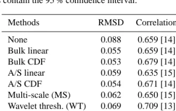
Table 1. RMSD (in units of m3m−3) and correlation between INS and AMS SM at Kyeamba treated by various methods. The square brackets contain the 95 % confidence interval.
Methods RMSD Correlation
None 0.088 0.659[14]
Bulk linear 0.055 0.659[14]
Bulk CDF 0.053 0.679[14]
A/S linear 0.059 0.635[15]
A/S CDF 0.054 0.671[14]
Multi-scale (MS) 0.062 0.650[15]
Wavelet thresh. (WT) 0.069 0.709[13]
WT+MS 0.048 0.711[12]
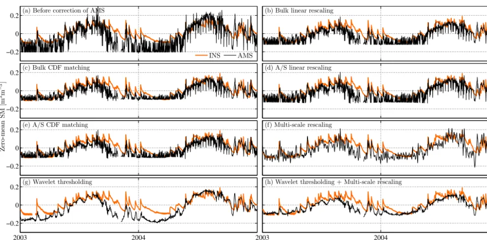
suppression of the associated signal, as well as noise, com-ponents: std(Yj∗)<std(Yj), and std(Y∗,j)<std(Y,j). For AMS, the bulk linear scheme corrects the coarse-scale bias inY8(a)component and rescales the noise variance, reducing RMSD from 0.09 to 0.06 m3m−3. However, the fine-scale biases inYj∗are still present, and increased on some scales, e.g. atj=4, 7 for AMS∗. Additionally for A/S linear rescal-ing,R(AMS∗,INS) value does not change significantly and the noise are still clearly visible in Fig. 6b and d.
By construction, the MS rescaling uses the estimatedαˆY,j
values from Fig. 5a to correct bias on all the scales. Fig. 5f
shows the analysis of MS-corrected Y∗. The equivalence ˆ
αY∗,j=1 indicates that the multiplicative biases are elimi-nated atj >2. At j=1–2, as the scaling coefficients can-not be estimated by TC, CDF matching was applied to these scales such that the biases are still present on these scales. Amid the reduction of biases, we also observed noise ampli-fication (i.e. std(Y∗,j)>std(Y,j)) in AMS∗atj=3, 7 and in MER∗atj=3–7, because of rescaling with less-than-unity
ˆ
αY,j values in Eq. (10). Indeed it is evident from Eq. (6) that
it is possible to increase the noise variance and MSE when reducing the bias component of the MSE. This in turn leads to larger disagreement between INS and AMS in terms of RMSD andR, and the increased amplitudes of the noise ob-served in AMS in Fig. 6f.
The bulk and A/S CDF methods produced very similar re-sults with each other, and also with their linear counterparts. There is signal and noise suppression, but the scale-level bi-ases are retained. The signal components ofY∗are negatively biased atj=3–7 and positively biased atj=8. The CDF-corrected AMS∗ shows slightly better RMSD and R with INS, owing to the reduced noise variance and a reduced bias at AMS(8a)∗.
[image:9.612.78.257.445.558.2]im-−0.2 0
0.2(a) Before correction of AMS
Ze
ro
-m
ea
n
S
M
[m
3m
−
3]
INS AMS
(b) Bulk linear rescaling
−0.2 0
0.2(c) Bulk CDF matching (d) A/S linear rescaling
−0.2 0
0.2(e) A/S CDF matching (f) Multi-scale rescaling
2003 2004
−0.2 0
0.2(g) Wavelet thresholding
Time [year] 2003 2004
(h) Wavelet thresholding + Multi-scale rescaling
[image:10.612.53.548.64.308.2]Time [year]
Figure 6. Time series of AMS SM at Kyeamba treated by various bias correction schemes. The use of WT-based de-noising has also been
demonstrated in (g, h).
provements in RMSD and correlation between the corrected
Y∗ and the referenceX are somewhat superficial, masking the fact that the bias correction is limited to the coarsest scales. On the other hand, the A/S-based and MS methods can modify the original noise profiles in the data across the scales, by amplifying (or suppressing) noise in individual components (either Yj,YS, orYA) with less-than
(greater-than) unity pre-correction α. This may be considered unde-sirable for an objective to produce more physically represen-tative data with a simple error structure on the whole. There-fore, arguably, none of these methods is entirely satisfactory, in manners of not removing the multiplicative biases com-pletely and/or changing error characteristics. From this view-point, the task of bias correction is seen as inseparable from that of noise reduction when considering MS (or A/S) bias correction, unless certain components in MRA were explic-itly ignored.
7 Combining bias correction with wavelet de-noising The last example presents an impetus to consider noise re-moval prior to bias correction and produce a simpler error structure in the bias-corrected data Y∗. Critically, TC pro-vides noise and signal estimates that can be used for de-noising through thresholding of wavelet coefficientspj k. The
basic rationale for wavelet thresholding (WT) is that inicant detail coefficients are likely due to noise, while signif-icant ones are related to the signal component. Thus, a co-efficient is eliminated if its magnitude is less than a given
thresholdλp; otherwise, it is modified according to a trans-formation function 0(pj k) to remove the influence of the noise (Donoho and Johnstone, 1994).
One commonly used transformation is soft thresholding (Donoho, 1995), where the coefficients are modified accord-ing to
0λp pj k
=
sign pj kmax |pj k−λp|,0. (11)
Such de-noising filters have near-optimal properties in the minmax sense. We follow the BayesShrink rule of Chang et al. (2000) to define a set of scale-dependent threshold val-ues using
λp,j= var p,j
αp,jstd fj
, (12)
Y∗= Y 0
ˆ
αY0 + j0
X
j=1 nj
X
k=1
0λp,j Yj k
ˆ
αY,j
ψj k. (13)
The prescription, which is essentially a two-stage opera-tion, was applied to AMS for comparisons with the previous results. The first stage of de-noising leads to smoothing of the time series, improved Rwith INS by 0.05, and reduced RMSD by 0.02 m3m−3. The actual SM variability has be-come more apparent in Fig. 6g. Over-smoothing can occur due to our inability to properly distinguish signal from noise in AMS1 and AMS2 where the signal-to-noise ratio is very
low. However, without the second stage of bias correction, the dynamic ranges of de-noised AMS and INS are visibly different, such that the improvement in RMSD with INS is limited. Combining WT and MS leads to improvement in both metrics of RMSD=0.048 m3m−3andR=0.711, with Fig. 6h confirming that the reduced noise was not amplified by the MS rescaling.
8 Conclusions
This work combines MRA and TC in a new analysis frame-work with increased capacity to provide a more compre-hensive view of the inter-data relations on short and long timescales. TC (or CDF) rescaling can be exploited on in-dividual scales to reduce scale-specific multiplicative biases, and provide “prior” knowledge of noise for calibrating a WT-based de-noising filter. As a demonstration of principle, these methods are applied to SM data from in situ and satellite sen-sors and a land surface model. Using MRA, we found that the three data exhibit significantly different wavelet spectra and variable degrees of agreement on different timescales. On fine scales, the contribution of noise is most prominent, un-dermining the correlation between the data sets. By contrast, the biases are most apparent on coarse scales. Furthermore, these biases are non-systematic across timescales in the study region and across spatial locations over Australia, and the signal-to-noise ratios vary with scales and between the vari-ous data, pointing to the need to use correction schemes that are capable of handling such complexities.
Appendix A: Wavelet statistical analysis
MRA enables the (bulk) variance var(p) of a time seriespto be decomposed into wavelet variances var(pj) on different
scalesj. Analogous to a Fourier spectrum, the expansion of var(p) yields a wavelet spectrum and is given by
var(p)=
J X
j=1
var pj (A1)
=varp(ja)
0
+
j0
X
j=1
var pj
(A2)
where the variance of the approximation time seriesp(ja)
0 can
be expressed in terms of that of the detail time seriespj. Similarly, wavelet covariance cov(Xj,Yj) at a givenj in-dicates the contribution of covariance between two time se-ries (X,Y) on that scale. Specifically, the wavelet covariance on scalej can be expressed as
cov Xj, Yj= 1
nj nj
X
k=1
Xj kYj k, (A3)
noting that there is an equivalence of computing (co)variance in the wavelet and time domains. To exclude the boundary influence of a finite-length time series and missing values in the time series, an estimator of the wavelet covariance can be constructed by excluding the coefficients affected by the boundaries and gaps, followed by renormalisation. In the pa-per, we find it more intuitive to report the wavelet correlation, namely
R Xj, Yj=
cov Xj, Yj
q
var Xjvar Yj
. (A4)
Appendix B: Multi-scale triple collocation
Starting with the scale-level affine model of Eqs. (4) and (5), the associated scaling coefficients (α0p,αp,j) and error
vari-ances (var(p0), var(p,j)) for each scale can be estimated
us-ing TC. We use solutions of Su et al. (2014a) for the data tripletp= {X, Y, Z}on each scale separately: withXas the reference by settingαX,j,αX0 =1,
ˆ
αY,j = cov Yj, Zj
cov Xj, Zj
, (B1)
ˆ
αZ,j=
cov Yj, Zj
cov Xj, Yj, (B2)
ˆ var p,j
=var pj
−cov pj, qj
cov pj, rj
cov qj, rj
, (B3)
ˆ var fj
=var Xj
−var p,j
(B4) whereq andr are also data labels, butp6=q6=r. The hat notation is used throughout the paper to distinguish esti-mates from true values. It can be shown that, in proba-bility, TC yields unbiased estimates whereby αp,jˆ =αp,j,
ˆ
var(p,j)=var(p,j), and varˆ (fj)=var(fj). These expres-sions were used to compute the results in Fig. 5 and the threshold values for wavelet de-noising. When TC does not produce physically meaningful estimates from negative or small covariance due to weak instruments and possible in-adequacy of the considered signal and noise model, the OLS estimator was used,
ˆ
αY,jOLS=cov Xj, Yj
var Xj
, (B5)
although its estimates are biased (αˆY,jOLS< αY,j) for our
pur-pose, due to the extraneous contribution of noise variance in the denominator. Similarly the VAR estimator can be used,
ˆ
αY,jVAR=p
Acknowledgements. We thank Wade Crow for valuable
dis-cussions and Clara Draper for her critiques of the early drafts. We acknowledge gratefully the feedback of Simon Zwieback, two anonymous reviewers, Wolfgang Wagner, and Editor Niko Verhoest in the refinement of our manuscript. We also thank all who contributed to the data sets used in this study. Kyeamba in situ data were produced by colleagues at Monash University and the University of Melbourne who have been involved in the OzNet programme. AMSR-E data were produced by Richard de Jeu and colleagues at Vrije University Amsterdam and NASA. The MERRA-Land data set was provided by NASA Goddard Earth Sciences Data and Information Services Center (GES DISC). The land cover/use map was produced by merging land cover (Lymburner et al., 2010) and land use (Australian Bureau of Rural Science, 2010) data sets. The recalibrated precipitation data of the Australian Water Availability Project (AWAP) (Jones et al., 2009) were obtained from the Australian Bureau of Meteorology. National soil data (McKenzie et al., 2005) were provided by the Australian Collaborative Land Evaluation Program ACLEP, endorsed through the National Committee on Soil and Terrain NCST (http://www.clw.csiro.au/aclep). The 9 s digital elevation map is obtained from Geoscience Australia (2008). This research was conducted with financial support from the Australian Research Council (ARC Linkage Project No. LP110200520) and the Bureau of Meteorology, Australia.
Edited by: N. Verhoest
References
Albergel, C., De Rosnay, P., Gruhier, C., Muñoz-Sabater, J., Hase-nauer, S., Isaksen, L., Kerr, Y., and Wagner, W.: Evaluation of re-motely sensed and modelled soil moisture products using global ground-based in situ observations, Remote Sens. Environ., 118, 215–226, doi:10.1016/j.rse.2011.11.017, 2012.
Australian Bureau of Rural Science: Land Use of Australia, version 4, 2005/2006, available at: http://data.daff.gov.au/ anrdl/metadata_files/pa_luav4g9abl07811a00.xml (last access: 24 July 2014), 2010.
Brocca, L., Moramarco, T., Melone, F., Wagner, W., Hasenauer, S., and Hahn, S.: Assimilation of surface- and root-zone ASCAT soil moisture products into rainfall–runoff modeling, IEEE T. Geosci. Remote, 50, 2542–2555, doi:10.1109/TGRS.2011.2177468, 2012.
Caires, S. and Sterl, A.: Validation of ocean wind and wave data using triple collocation, J. Geophys. Res., 103, 3098, doi:10.1029/2002JC001491, 2003.
Chang, S. G., Yu, B., and Yeterli, M.: Adaptive wavelet thresholding for imaging denoising and compression, IEEE T. Image Process., 9, 1532–1546, doi:10.1109/83.862633, 2000.
Daubechies, I.: Ten Lectures on Wavelets, Society for Industrial and Applied Mathematics, doi:10.1137/1.9781611970104, 1992. Donoho, D. L.: Denoising via soft thresholding, IEEE T. Inform.
Theory, 41, 613–627, doi:10.1109/18.382009, 1995.
Donoho, D. L. and Johnstone, I. M.: Ideal spatial adap-tion via wavelet shrinkage, Biometrika, 81, 425–455, doi:10.1093/biomet/81.3.425, 1994.
Draper, C., Reichle, R., De Lannoy, G., and Liu, Q.: Assimilation of passive and active microwave soil moisture retrievals, Geophys. Res. Lett., 39, L04401, doi:10.1029/2011GL050655, 2012. Draper, C. S., Reichle, R. R., de Jeu, R. A., Naeimi, V.,
Pari-nussa, R. M., and Wagner, W.: Estimating root mean square er-rors in remotely sensed soilmoisture over continental scale do-mains, Remote Sens. Environ., 137, 288–298, doi:10.1175/JHM-D-12-052.1, 2013.
Drusch, M., Wood, E. F., and Gao, H.: Observation opera-tors for the direct assimilation of TRMM microwave im-ager retrieved soil moisture, Geophys. Res. Lett., 32, L15403, doi:10.1029/2005GL023623, 2005.
Entin, J. K., Robock, A., Vinnikov, K. Y., Hollinger, S. E., Liu, S., and Namkhai, A.: Temporal and spatial scales of observed soil moisture variations in the extratropics, J. Geophys. Res., 105, 11865–11877, doi:10.1029/2000JD900051, 2000.
Garcia, D.: Robust smoothing of gridded data in one and higher dimensions with missing values, Comput. Stat. Data Anal., 54, 1167–1178, doi:10.1016/j.csda.2009.09.020, 2010.
Geoscience Australia: GEODATA 9-Second DEM Version 3, available at: http://www.ga.gov.au/metadata-gateway/metadata/ record/66006/ (last access: 24 July 2014), 2008.
GLACE Team, Koster, R. D., Dirmeyer, P. A., Guo, Z., Bo-nan, G., and Chan, E.: Regions of strong coupling between soil moisture and precipitation, Science, 305, 1138–1140, doi:10.1126/science.1100217, 2004.
Gruber, A., Dorigo, W. A., Zwieback, S., Xaver, A., and Wagner, W.: Characterizing Coarse-Scale Representative-ness of in situ Soil Moisture Measurements from the In-ternational Soil Moisture Network, Vadose Zone J., 12, doi:10.2136/vzj2012.0170, 2013.
Janssen, P. A. E. M., Abdalla, S., Hersbach, H., and Bid-lot, J.-R.: Error estimation of buoy, satellite, and model wave height data, J. Atmos. Ocean. Tech., 24, 1665–1677, doi:10.1175/JTECH2069.1, 2007.
Jones, D. A., Wang, W., and Fawcett, R.: High-quality spatial cli-mate data-sets for Australia, Aust. Meteorol. Oceanogr., 58, 233– 248, 2009.
Koster, R. D., Guo, Z., Yang, R., Dirmeyer, P. A., Mitchell, K., and Puma, M. J.: On the nature of soil moisture in land surface mod-els, J. Climate, 22, 4322–4335, doi:10.1175/2009JCLI2832.1, 2009.
Kumar, S. V., Reichle, R. H., Harrison, K. W., Peters-Lidard, C. D., Yatheendradas, S., and Santanello, J. A.: A comparison of meth-ods for a priori bias correction in soil moisture data assimilation, Water Resour. Res., 48, W03515, doi:10.1029/2010WR010261, 2012.
Legates, D. R., Mahmood, R., Levia, D. F., DeLiberty, T. L., Quir-ing, S. M., Houser, C., and Nelson, F. E.: Soil moisture: a central and unifying theme in physical geography, Prog. Phys. Geogr., 35, 65–86, doi:10.1177/0309133310386514 , 2011.
Liu, Y. Y., Dorigo, W. A., Parinussa, R. M., De Jeu, R. A. M., Wagner, W., McCabe, M. F., Evans, J. P., and Van Dijk, A. I. J. M.: Trend-preserving blending of passive and active microwave soil moisture retrievals, Remote Sens. Environ., 123, 280–297, doi:10.1016/j.rse.2012.03.014, 2012.
Lymburner, L., Tan, P., Mueller, N., Thackway, R., Lewis, A., Thankappan, M., Randall, L., Islam, A., and Senarath, U.: 250 metre Dynamic Land Cover Dataset of Australia, 1st Edn., Geoscience Australia, Canberra, 2010.
Mallat, S. G.: A theory for multiresolution signal decomposition: the wavelet representation, IEEE T. Pattern Anal., 11, 674–693, doi:10.1109/34.192463, 1989.
McKenzie, N. J., Jacquier, D. W., Maschmedt, D. J., Griffin, E. A., and Brough, D. M.: The Australian Soil Resource Information System: Technical Specifications, National Committee on Soil and Terrain Information/Australian Collaborative Land Evalua-tion Program, Canberra, 2005.
Miralles, D. G., De Jeu, R. A. M., Gash, J. H., Holmes, T. R. H., and Dolman, A. J.: Magnitude and variability of land evaporation and its components at the global scale, Hydrol. Earth Syst. Sci., 15, 967–981, doi:10.5194/hess-15-967-2011, 2011.
Mittelbach, H. and Seneviratne, S. I.: A new perspective on the spatio-temporal variability of soil moisture: temporal dynamics versus time-invariant contributions, Hydrol. Earth Syst. Sci., 16, 2169–2179, doi:10.5194/hess-16-2169-2012, 2012.
Owe, M., de Jeu, R., and Holmes, T.: Multisensor historical clima-tology of satellite-derived global land surface moisture, J. Geo-phys. Res., 113, F01002, doi:10.1029/2007JF000769, 2008. Peel, M. C., Finlayson, B. L., and McMahon, T. A.: Updated
world map of the Köppen–Geiger climate classification, Hy-drol. Earth Syst. Sci., 11, 1633–1644, doi:10.5194/hess-11-1633-2007, 2007.
Reichle, R. H. and Koster, R. D.: Bias reduction in short records of satellite soil moisture, Geophys. Res. Lett., 31, L19501, doi:10.1029/2004GL020938, 2004.
Reichle, R. H., Koster, R. D., Dong, J., and Berg, A. A.: Global soil moisture from satellite observations, land sur-face models, and ground data: implications for data as-similation, J. Hydrometeorol., 5, 430–442, doi:10.1175/1525-7541(2004)005<0430:GSMFSO>2.0.CO;2, 2004.
Reichle, R. H., Koster, R. D., Liu, P., Mahanama, S. P. P., Njoku, E. G., and Owe, M.: Comparison and assimila-tion of global soil moisture retrievals from the Advanced Microwave Scanning Radiometer for the Earth Observ-ing System (AMSR-E) and the ScannObserv-ing Multichannel Mi-crowave Radiometer (SMMR), J. Geophys. Res., 112, D09108, doi:10.1029/2006JD008033, 2007.
Reichle, R. H., Koster, R. D., De Lannoy, G. J. M., Forman, B. A., Liu, Q., Mahanama, S. P. P., and Touré, A.: Assessment and en-hancement of MERRA land surface hydrology estimates, J. Cli-mate, 24, 6322–6338, doi:10.1175/JCLI-D-10-05033.1, 2011. Rienecker, M. M., Suarez, M. J., Gelaro, R., Todling, R.,
Bacmeis-ter, J., Liu, E., Bosilovich, M. G., Schubert, S. D., Takacs, L., Kim, G.-K., Bloom, S., Chen, J., Collins, D., Conaty, A., da Silva, A., Gu, W., Joiner, J., Koster, R. D., Lucchesi, R., Molod, A., Owens, T., Pawson, S., Pegion, P., Redder, C. R., Reichle, R., Robertson, F. R., Ruddick, A. G., Sienkiewicz, M., and Woollen, J.: MERRA – NASA’s Modern-Era Retrospective Analysis for Research and Applications, J. Climate, 24, 3624– 3648, doi:10.1175/JCLI-D-11-00015.1, 2011.
Rodrigeuz-Iturbe, I.: Ecohydrology: a hydrologic perspective of climate-soil-vegetation dynamics, Water Resour. Res., 36, 3–9, doi:10.1029/1999WR900210, 2000.
Roebeling, R. A., Wolters, E. L. A., Meirink, J. F., and Leijnse, H.: Triple collocation of summer precipitation retrievals from SE-VIRI over Europe with gridded rain gauge and weather radar data, J. Hydrometeorol., 13, 1552–1566, doi:10.1175/JHM-D-11-089.1, 2013.
Scipal, K., Drusch, M., and Wagner, W.: Assimilation of a ERS scat-terometer derived soil moisture index in the ECMWF numerical weather prediction system, Adv. Water Resour., 31, 1101–1112, doi:10.1016/j.advwatres.2008.04.013, 2008a.
Scipal, K., Holmes, T., de Jeu, R., Naeimi, V., and Wagner, W.: A possible solution for the problem of estimating the error struc-ture of global soil moisstruc-ture data sets, Geophys. Res. Lett., 35, L24403, doi:10.1029/2008GL035599, 2008b.
Smith, A. B., Walker, J. P., Western, A. W., Young, R. I., El-lett, K. M., Pipunic, R. C., Grayson, R. B., Siriwardena, L., Chiew, F. H. S., and Richter, H.: The Murrumbidgee soil moisture network data set, Water Resour. Res., 48, W07701, doi:10.1029/2012WR011976, 2012.
Steelman, C. M., Endres, A. L., and Jones, J. P.: High-resolution ground penetrating radar monitoring of soil moisture dy-namics: Field results, interpretation, and comparison with unsaturated flow model, Water Resour. Res., 48, W09538, doi:10.1029/2011WR011414, 2012.
Stoffelen, A.: Towards the true near-surface wind speed: Error mod-elling and calibration using triple collocation, J. Geophys. Res., 103, 7755–7766, doi:10.1029/97JC03180, 1998.
Su, C.-H., Ryu, D., Young, R. I., Western, A. W., and Wagner, W.: Inter-comparison of microwave satellite soil moisture retrivals over Murrumbidgee Basin, southeast Australia, Remote Sens. Environ., 134, 1–11, doi:10.1016/j.rse.2013.02.016, 2013a. Su, C.-H., Ryu, D., Western, A. W., and W. Wagner, W.: De-noising
of passive and active microwave satellite soil moisture time se-ries, Geophys. Res. Lett., 40, 3624–3630, doi:10.1002/grl.50695, 2013b.
Su, C.-H., Ryu, D., Crow, W. T., and Western, A. W.: Beyond triple collocation: applications to satellite soil moisture, J. Geophys. Res.-Atmos., 119, 6419–6439, doi:10.1002/2013JD021043, 2014a.
Su, C.-H., Ryu, D., Crow, W. T., and Western, A. W.: Stand-alone error characterisation of microwave satellite soil moisture us-ing a Fourier method, Remote Sens. Environ., 154, 115–126, doi:10.1016/j.rse.2014.08.014, 2014b.
Wang, G., Garcia, D., Liu, Y., de Jeu, R., and Dolman, A. J.: A three-dimensional gap filling method for large geo-physical datasets: application to global satellite soil mois-ture observations, Environ. Modell. Softw., 30, 139–142, doi:10.1016/j.envsoft.2011.10.015, 2012.
Western, A. W., Grayson, R. B., and Bloschl, G.: Scaling of soil moisture: a hydrologic perspective, Annu. Rev. Earth Pl. Sc., 30, 149–180, doi:10.1146/annurev.earth.30.091201.140434, 2002. Wright, P. G.: The Tariff on Animal and Vegetable Oils, Macmillan,
New York, 1928.
Zwieback, S., Scipal, K., Dorigo, W., and Wagner, W.: Struc-tural and statistical properties of the collocation technique for error characterization, Nonlin. Processes Geophys., 19, 69–80, doi:10.5194/npg-19-69-2012, 2012.