www.hydrol-earth-syst-sci.net/18/2695/2014/ doi:10.5194/hess-18-2695-2014
© Author(s) 2014. CC Attribution 3.0 License.
Large-scale analysis of changing frequencies of rain-on-snow events
with flood-generation potential
D. Freudiger, I. Kohn, K. Stahl, and M. Weiler
Chair of Hydrology, University of Freiburg, Freiburg, Germany
Correspondence to: D. Freudiger ([email protected])
Received: 18 September 2013 – Published in Hydrol. Earth Syst. Sci. Discuss.: 5 November 2013 Revised: 21 May 2014 – Accepted: 27 May 2014 – Published: 24 July 2014
Abstract. In January 2011 a rain-on-snow (RoS) event caused floods in the major river basins in central Europe, i.e. the Rhine, Danube, Weser, Elbe, Oder, and Ems. This event prompted the questions of how to define a RoS event and whether those events have become more frequent. Based on the flood of January 2011 and on other known events of the past, threshold values for potentially flood-generating RoS events were determined. Consequently events with rainfall of at least 3 mm on a snowpack of at least 10 mm snow wa-ter equivalent (SWE) and for which the sum of rainfall and snowmelt contains a minimum of 20 % snowmelt were anal-ysed. RoS events were estimated for the time period 1950– 2011 and for the entire study area based on a temperature index snow model driven with a European-scale gridded data set of daily climate (E-OBS data). Frequencies and magni-tudes of the modelled events differ depending on the eleva-tion range. When distinguishing alpine, upland, and lowland basins, we found that upland basins are most influenced by RoS events. Overall, the frequency of rainfall increased dur-ing winter, while the frequency of snowfall decreased durdur-ing spring. A decrease in the frequency of RoS events from April to May has been observed in all upland basins since 1990. In contrast, the results suggest an increasing trend in the magni-tude and frequency of RoS days in January and February for most of the lowland and upland basins. These results suggest that the flood hazard from RoS events in the early winter sea-son has increased in the medium-elevation mountain ranges of central Europe, especially in the Rhine, Weser, and Elbe river basins.
1 Introduction
Rain-on-snow (RoS) events are relevant for water resources management, particularly for flood forecasting and flood risk management (McCabe et al., 2007). RoS events have the potential to cause large flood events during the winter sea-son. They represent one of five flood process types defined by Merz and Blöschl (2003) that occur in temperate-climate mountain river systems and are strongly elevation dependent. These events are complex as they do not only depend on the rain intensity and amount, but also on the prevailing freez-ing level, the snow water equivalent (SWE), the snow en-ergy content, the timing of release, and the areal extent of the snowpack (Kattelmann, 1997; McCabe et al., 2007). Snow-packs are water reservoirs of large regional extent and storage capacity, which can produce rapid melt in combination with warm air temperatures and high humidity (e.g. Singh et al., 1997; Marks et al., 1998). Consequently, cumulative rainfall and snowmelt can increase the magnitude of runoff and can thus generate much greater potential for flooding than a usual snowmelt event (Kattelmann, 1985; Marks et al., 1998). Be-sides their large damage potential, such events are also very difficult to forecast as shown by Rössler et al. (2014) for a RoS-driven flood event in October 2011 in the Bernese Alps in Switzerland. Scientific interest has therefore increased in the last decades, and a number of different methods of analy-sis have been developed to better understand and quantify the physical processes by studying individual events in different locations (e.g. Blöschl et al., 1990; Singh et al., 1997; Floyd and Weiler, 2008; Garvelmann et al., 2013).
a more variable snow- and rain-fed regime in the future in Switzerland. These meteorological changes are very likely to influence the occurrence and magnitude of RoS events, and Köplin et al. (2014) predict a diversification of flood types in the wintertime as well as an increase of RoS flood events in the future in Switzerland.
Although Merz and Blöschl (2003) observed that 20 % of the flood events in Austria were RoS-driven during the period 1971–1997 and hence showed the importance of such events in central Europe, only few studies have specifically anal-ysed the changes of the frequency of RoS events over time and especially over large areas. Ye et al. (2008) observed an increase in RoS days in northern Eurasia, which they were able to correlate with the observed increase in air tempera-ture and rainfall in the wintertime. Sui and Koehler (2001) attributed an increase in peak flows in the northern Danube tributaries in Germany to an increase in RoS events, based on the combination of decreasing SWE and increasing maxi-mum daily winter precipitation sums they found at a number of climate stations in the area. McCabe et al. (2007) found disparate trends in the western USA with generally positive temporal trends of RoS events frequencies for high-elevation sites and negative trends for low-elevation sites. In these ar-eas, the increase of temperature appears to affect the occur-rence of snow, contributing therefore to a lower frequency of RoS events (McCabe et al., 2007). Similarly, Surfleet and Tullos (2013) predicted with a model experiment that an in-crease in air temperature due to climate change would lead to a decrease of high peak flow due to RoS events for low- and middle-elevation zones, while at high-elevation bands these kinds of events would increase. All these studies show the correlation between the frequency of RoS events, the changes in air temperature, and the importance of the elevation range. They therefore stress the need for a more accurate trend anal-ysis of those events in the context of climate change in cen-tral Europe, where discharges mainly depend on alpine and mid-elevation tributaries.
Previous studies differ on the definition of RoS events. McCabe et al. (2007) and Surfleet and Tullos (2013) de-fined an event as RoS-driven if simultaneously rainfall oc-curs, maximum daily temperature is greater than 0◦C, and a decrease in snowpack can be observed; while for Ye et al. (2008), a RoS event takes place only when at least one of four daily precipitation measurements is liquid and the ground is covered by ≥1 cm of snow. Sui and Koehler (2001) found that most RoS events in southern Germany occurred when snowmelt was larger than the rainfall depth. These definitions allow identifying all possible RoS events but are insufficient if one focusses on the events that can effectively cause flood events.
Due to the great hydrologic impact that RoS events can have, there is a real need for assessing the changes in fre-quencies of those RoS events that may generate large floods. A good example of such an event is the flood in January 2011 in central Europe. During a strong negative phase of the
North Atlantic Oscillation, temperature anomalies in De-cember 2010 reached –4◦C in central and northern Europe
(Lefebvre and Becker, 2011), and record snowpacks were ob-served nearly all over Germany for this time of the year (e.g. Böhm et al., 2011; LHW, 2011; Besler, 2011). January 2011 then brought thawing temperatures in combination with rain-fall events, and from 6 to 16 January very high flows were observed at nearly all German gauging stations (e.g. Böhm et al., 2011; Bastian et al., 2011; Karuse, 2011; LHW, 2011; Fell, 2011; Besler, 2011). Kohn et al. (2014) identified the si-multaneous occurrence of rainfall and snowmelt as the driv-ing factor for those flood events, which led, beside other im-pacts, to a restriction of navigation on the river Rhine and large inundations in the lower Elbe river basin. The aims of this study are therefore (i) to derive criteria for RoS-driven events that have the potential to cause floods, using the case study of January 2011 in Germany, and (ii) to analyse the changes in frequencies and magnitudes of these types of events during the time period 1950–2011 in six major cen-tral European river basins, i.e. Rhine, Danube, Elbe, Weser, Oder, and Ems.
2 Materials and methods 2.1 Study area
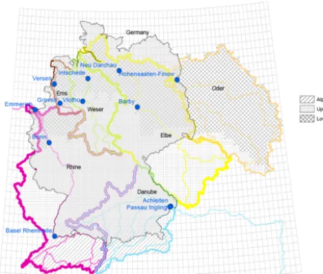
The study area embodies the six major river basins of the German fluvial network. Since only German streamflow records were used, the basins of the rivers Rhine, Danube, Elbe, Weser, Oder, and Ems are considered only upstream of the most downstream station in German territory (Fig. 1). Ac-cording to the Hydrological Atlas of Germany (HAD, Bun-desanstalt für Gewässerkunde), the basins were divided into alpine, upland, or lowland sub-basins. This classification is motivated by the elevation of the main tributaries, but is not strictly guided by elevation as the main rivers drop quickly to lower elevations.
Only the basins of the rivers Rhine and Danube have an “alpine” section in this classification. The alpine portion of the Rhine encompasses the basin ca. above Basel, and be-sides the entire basin area in Austria and Switzerland with high mountains up to 4000 m a.s.l.it also includes the south-ern Black Forest with elevations of only up to 1500 m a.s.l.
The alpine section of the Danube basin consists also of a small part in the Black Forest near the source, but then in-cludes mainly the southern tributaries of the Danube from the Alps. They comprise the river Inn, which originates from the Swiss and Austrian Alps with elevations over 3000 m a.s.l., as well as a number of tributaries from the northern range of the Alps along the German–Austrian border with elevations below 3000 m a.s.l.
Figure 1. Study area: delimitation of the basin boundaries of the
Rhine, Danube, Elbe, Weser, Oder, and Ems basins and subdivi-sion into alpine, upland, and lowland. The background raster corre-sponds to the E-OBS data set. Gauging stations at the outlet of each sub-basin are represented with blue dots.
northern part of the Czech Republic (Elbe basin). The land-scape can be described as upland with elevation ranges from 200–300 m a.s.l.to up to Feldberg, 1493 m a.s.l., the highest mountain in Germany outside the Alps.
With the exception of the Danube, which is only consid-ered to the German border, all river basins contain a low-land section. These areas in northern Germany and western Poland (Oder basin) are mainly constituted of lowland areas with altitudes ranging from 0 to 200 m a.s.l.
2.2 Meteorological and hydrometric data
Daily mean temperature and precipitation sums were ob-tained from the European Climate Assessment and Dataset project (ECA&D, http://www.ecad.eu) and the EU-FP6 project ENSEMBLES (http://ensembles-eu.metoffice.com). The so-called E-OBS data set (version 6.0) was interpolated from climate stations all across Europe into a 0.25◦×0.25◦ regular latitude–longitude grid (Fig. 1; Haylock et al., 2008). The time series are available from 1 January 1950 to 31 De-cember 2011 and cover the study area 46.00–55.25◦N, 5.25– 19.75◦E.
Daily mean discharge data from more than 300 gauging stations (Fig. 2) in Germany were provided by German pub-lic authorities. Details on the assembled data set can be found in Kohn et al. (2014). The time series are of different lengths, but most of them cover the period 1950–2011. Since author-ities usually correct peak discharge values with hydraulic modelling or revise rating curves during the years after a flood event, some of the most recent data used in this study were raw (as yet uncorrected) data. However, later
correc-tions to the peaks are not expected to change the relative ranking and hence the results of the trend analysis, and the discharge data were found suitable for this study. To assess the accuracy of the data, all data included in this analysis passed a visual quality control.
2.3 Estimation of snowpack and snowmelt
Snow accumulation and melt were estimated based on daily E-OBS mean temperature and precipitation sum data for the entire study area and are given in mm SWE. Precipitation is assumed to be solid if air temperatureTa<1◦C and liquid
ifTa≥1◦C. Snowmelt M (mm) is estimated using a
tem-perature index model, which assumes a relationship between ablation and air temperature (Eq. 1; e.g. Finsterwalder and Schunk, 1887; Collins, 1934; Corps of Engineers, 1956).
M=Mf·(Ta−Tb) (1)
Martinec and Rango (1986) calculated degree-day fac-tors Mf for open areas depending on the snow density
of the snowpack. They suggested Mf values from 3.5 to
6 mm◦C−1day−1 and even smaller for fresh snow. They also observed thatMfincreases over the melt period. Hock
(2003) listed Mf values for snow in high-elevation areas
between 2.5 and 6 mm◦C−1day−1. For sake of simplicity of the large-scale analysis, a constant conservative value of Mf=3 mm◦C−1day−1 was chosen for the entire study
area and melt period. This value was found to represent the area well, since snow melts very fast in upland and low-land regions in Germany and the snowpack consists there-fore mainly of fresh snow. The base temperatureTb
repre-sents the threshold temperature for melting snow. Most stud-ies setTbto 1◦C, since energy is needed to bring the snow
to 0◦C to start melting (e.g. Hock, 2003).T
bwas therefore
set to 1◦C. The sensitivity of the subsequent trend
calcula-tion to the choice ofTb andMf was tested ranging from 0
to 2◦C forTband from 2 to 5 mm◦C−1day−1forMf. Both
parameters were found to have an impact on the calculated snow depth but to be rather insensitive for the trends calcu-lation, since the trend analysis considers relative changes to the mean (Kohn et al., 2014).
For every grid cell, daily SWE of the snowpack was cal-culated for dayias the sum of the SWE of the day before and the snowmeltM(mm) or snowfallS(mm SWE) of the actual day (Eq. 2) and is given in mm SWE.
SWEi= (
SWEi−1+Si, if Ta< Tb
SWEi−1−Mi, if Ta≥Tb
(2)
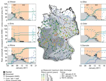
Figure 2. Large-scale analysis of the RoS event of January 2011. (a–f) Mean basin-wide daily snowpack, rainfall, and snowmelt (mm SWE)
from 1 to 31 January, as well as the percentage of snow-covered cells. Map: return period and occurrence period of the maximum daily discharge in the calender year 2011 at all gauging stations (modified from Kohn et al., 2014).
from 1 November to 31 May taking into account potential snow season extents in the entire study area. As snow mea-surements in Germany are available in few locations only, the calculated SWE was compared by (Kohn et al., 2014) to the products of the snow model SNOW4 (Germany’s National Weather Service, DWD), which is based on the interpolation of ground-based snow measurements, for the winter 2010– 2011. A frequency analysis was performed on the occurrence and amount of snow per area every day, and both model out-puts were found to be very similar.
2.4 Definition of RoS events
The aim of this study is to identify those RoS events in time series of rainfall occurrence and snowpack existence that have the potential to cause floods. Thus selection criteria need to be defined. The general variables for a RoS-driven runoff generation event are as follows:
1. RainfallR: the amount ofRmust be substantial, other-wise the event may be only snowmelt-driven.
2. Snowpack SWE: SWE needs to be large enough to be able to substantially contribute to runoff.
3. SnowmeltM: the amount ofM must be large enough compared toR; otherwise the event may be rather rain-driven.
The time and magnitude of a flood driven by a RoS event also depend on the response time of a basin. In this study we distinguish between a RoS day and a RoS event. A RoS day is defined as a day when all hydrometeorologic conditions (R, SWE, andM) for a RoS event are met. A RoS event al-ways starts with a RoS day and may contain RoS days and non-RoS days. A RoS event lasts from the initial RoS day to the day when the maximum discharge is observed after the first or after additional RoS days and within an assumed maximum response time following a RoS day. A RoS event with several RoS days is then considered as one event, even if it consists of multiple flood waves. We then defined the equivalent precipitation depthPeqof an event as
correspond-ing to the sum of daily rainfall and snowmelt durcorrespond-ing the RoS event.
Table 1. Historical RoS events (sources: Wetterchronik, 2001; Kohn et al., 2014).
Date Province Basin Event description
18 Mar 1970 Lower Saxony Elbe Snowmelt and rainfall led to flooding all over the river, especially in Uelzen and Lüneburg.
27–28 Feb 1987 Bavaria Danube Large flooding due to snowmelt and incessant rainfalls in Schambachtal.
20 Jan 1997 Rhineland-Palatinate Rhine Small flooding after a snow-rich January and a very wet February.
6–10 Jan 2011 Central Europe Western basins: First wave of large-scale flooding due to snow-rich December 2010 Rhine, Weser, Ems followed by thawing temperatures in January 2011.
11–16 Jan 2011 Central Europe All basins Second wave of large-scale flooding due to snow-rich December 2010 followed by thawing temperatures in January 2011.
the generalised extreme value distribution and the parame-ters were estimated with the maximum likelihood method (Venables and Ripley, 2002). This allowed proving the im-portance of the associated flood peaks. To clearly identify the flood event as RoS-driven, the measured peak discharge dur-ing the event was then compared to rainfall, modelled snow depth, and modelled snowmelt for each sub-basin, which al-lowed defined threshold values for R, SWE, andM. Addi-tionally, documented historical events, for which RoS pro-cesses were identified in the literature as the main cause for flooding within the study area, are listed in Table 1. These kinds of events are overall not well documented and the information comes mostly from diverse textual information sources, but it gives us the location and the day of occurrence of past RoS floods. This information was used to “validate” the selection criteria for RoS events that have been set on the flood event of January 2011, since it allows checking if the criteria are representative for other past events.
To comparePeqwith the observed river discharge of RoS
events that caused floods at the sub-basin scale, 12 gauging stations were selected (Fig. 1). In the case of nested basins, the difference in discharge between the lower and upper sta-tion was considered. No discharge data were available for the Oder basin outside Germany; therefore only one station at the outlet of the lowland sub-basin was considered. Finally, the probability distribution of the daily discharge values was classified into quantiles for each month and sub-basin. This expression gives an overview of the seasonal anomaly of RoS-driven peak discharge values. The 0.5 quantile repre-sents the median, and the closer to 1 the quantile is, the higher is the discharge and the higher is its flood-generating poten-tial.
2.5 Trend analysis
For all alpine, upland, and lowland sub-basins, thePeq, the
corresponding observed peak discharge, as well as the other variables influencing the occurrence of RoS events – namely
R, S, SWE, and M – were analysed for temporal trends. These trends were calculated as the slope of a linear
regres-sion with time and are expressed in percent to the mean value of the time series. This allows comparing the importance of the changes in time in one basin with the changes in other basins. The statistical significance of the trends was tested at a 5 % significance level using the non-parametric Mann– Kendall test (Mann, 1945). Trends were calculated and com-pared for the time periods 1950–2011 and 1990–2011, here-after referred to as long-term and short-term trends.
3 Results
3.1 Reanalysis of the large-scale RoS event in January 2011 in central Europe
The return periods of January 2011 peak flows illustrate the severity of large-scale flooding across Germany (Fig. 2g). Maximum annual daily discharge was observed from 6 to 16 January at all gauging stations except in the northern part of the Elbe lowland basin and in the Danube alpine sub-basin. With few exceptions discharge peaks reached at least a 1–2-year flood level, with large areas being affected by 20– 50-year floods along the main rivers and a few exception with 100-year floods in headwaters. Since two distinct dis-charge peaks were observed at nearly all gauging stations, the flood can be described as a two-wave flood event that spread from west to east. Figure 2a–f further shows the evolution of the mean basin-wide dailyR, SWE, and the percentage of snow-covered grid cells in the Rhine, Danube, Elbe, Weser, Ems, and Oder river basins during the flood event. On 5 Jan-uary 2011, snow covered 100 % of the grid cells of the study area and the mean SWE varied from 25 mm (Ems) to 70 mm (Danube). The discharge peaks correspond very well to two phases of rainfall combined with snowmelt, and the event was therefore identified as a RoS-driven flood.
During the first flood wave (W1, from 6 to 10 January), mean basinR of 2–10 mm day−1fell on the western basins (Fig. 2a, c, d), while in the eastern basins R never ex-ceeded 2 mm day−1 (Fig. 2b, d, f). W1 generated in total
Peq between 51 and 71 mm in the western basins Rhine,
basins Danube, Elbe, and Oder. In both regions the snowmelt content in Peq exceeded 25 %. Rain and snowmelt played
an equally important role in the western basins, whereas snowmelt played the most important role in the eastern basins.
During the second wave (W2, from 11 to 16 January), mean basinRreached 0–10 mm day−1in the western basins and 2–17 mm day−1in the eastern basins. W2 generated in totalPeq between 27 and 48 mm in the western basins, and
between 49 and 26 mm in the eastern basins. On 10 January, most of the snow had already melted in the northwestern part of Germany and W2 was therefore rather rain-driven in this area, especially in the Ems river basin, where the second flood wave was only rain-driven since all snow was already melted at this time. However, the snowpack was still substan-tial at the time in central Germany. After W2, nearly all snow was melted in the Ems, Weser, and Oder basins. In the Rhine and Danube river basins, most of the remaining snow was located in the alpine region.
In Fig. 2a–f the cumulative Peqs are also compared for
all sub-basins according to their elevation classification. The alpine sub-basins of the Rhine and Danube produced on average 4 mm day−1 equivalent precipitation depth during W1 and W2, which was only half of the other sub-basins. However, on 13 January the cumulative equivalent precipi-tation depth increased by 21 mm in the Danube alpine sub-basin. The upland sub-basins reacted very strongly to the RoS events, withPeqof almost 25 mm day−1during W1 in
all basins and especially in the west. The Weser upland ar-eas were once again strongly affected during W2. After W2, nearly all the grid cells were free of snow. During W1 Peq
was mostly caused by snowmelt at all elevation ranges in the east and showed very similar reaction for all lowland and up-land sub-basins. W2 resulted in a very fast increase of the cumulativePeqwithin few days in the east, especially for the
Elbe and Danube upland sub-basins (Fig. 2b, f). The Weser and Ems lowland sub-basins, in the western half of Germany, were also strongly impacted during W1, since the amount of snow was substantial and unusual, and it had nearly com-pletely melted by the end of W1. W2 therefore had only little impact on these elevation ranges in these sub-basins (Fig. 2a, c). The Rhine basin usually has a lot of snow during the wintertime, due to its larger upland elevation ranges and the influence of its alpine part. For this reason, there were not many differences in the snowmelt processes of the Rhine lowland and upland sub-basins, and both elevation ranges were strongly impacted by both RoS flood waves.
3.2 Criteria for potentially flood-generating RoS events Selection criteria for RoS events that have the potential to cause floods were chosen based on the reanalysis of the RoS-driven flood event in January 2011 in central Europe (Sect. 3.1). At the beginning of each flood wave, W1 and W2, the average basin SWE had reached at least 10 mm in
all river basins but the Ems, where all snow was already melted after W1. The average basin rainfall depth was at least 2 mm, and the average basin snowmelt was at least 25 % ofPeq. We therefore chose conservative threshold values of
3 mm for rainfall, 10 mm SWE for snowpack, and 20 % for the snowmelt amount inPeqto define a RoS day. During the
2011 event, the longest flood wave lasted 6 days (W2), and therefore the maximum response time of all basins was set to 6 days. Thus, the duration of a RoS flood event is limited to 6 days after the last RoS day.
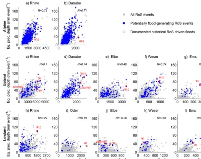
Figure 3 showsPeqfor all RoS events (R≥0 mm, SWE>
0 mm, M >0 %), potentially flood-generating RoS events according to the criteria above (R≥3 mm, SWE>10 mm,
M >20 %), and documented historical RoS-driven flood events against the corresponding measured discharge for all river sub-basins. Most of the sample “all events” have only little impact on the discharge and will not cause floods or are more rain-driven than rain-on-snow-driven and are therefore not of interest for this analysis. The selection of RoS events according to the above threshold values reveals that most of the RoS events in the alpine sub-basins have the poten-tial to generate floods, while in the lowland sub-basins only few events fall into this category. The criteria R≥3 mm, SWE>10 mm, andM >20 % were able to select all doc-umented historical RoS-driven flood events (Table 1) except for those of W1 in the lowland sub-basins of Oder and Elbe in January 2011. Less than 3 mm of rain fell in total, while the high temperatures generated more than 25 mm of snowmelt in these sub-basins. Thus, W1 was rather snowmelt-driven than driven in the lowland sub-basins, but it was RoS-driven at the scale of the whole Oder and Elbe basins.
Figure 3 also gives the correlation coefficients betweenPeq
and the corresponding measured peak discharges for each sub-basin. The correlation shows how strongly runoff gener-ation is RoS-driven. The higher the correlgener-ation, the more the discharge is influenced by RoS events. The alpine and up-land sub-basins of the Rhine, Weser, and Danube showed the highest positive correlation, with coefficients between 0.68 and 0.75. In the other upland sub-basins Elbe and Ems, cor-relation coefficients of 0.48 and 0.51 were found, and in all lowland sub-basins none of the correlation coefficients was higher than 0.48. A few large events in Fig. 3h–l suggest that a RoS event can emphasise a flood event if discharge is al-ready high at the time of occurrence.
Figure 3. Total equivalent precipitation depth and corresponding peak discharge for all possible RoS events (SP>0 mm SWE,M >0 %,
PL≥0 mm), for all potentially flood-generating events (SP>10 mm SWE,M >20 %,PL≥3 mm), and for documented historical
RoS-driven floods. The correlation coefficientRis given for the potentially flood-generating RoS events.
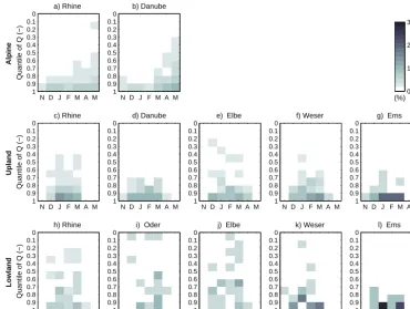
sub-basins, RoS events occurred from December to April, with most events in January–March again in the highest dis-charge class (quantiles of 0.9–1). Only few events corre-spond to discharge quantiles <0.7, confirming the strong flood-generating potential of the selected RoS events in this elevation range. In the lowland sub-basins, correspondence between RoS events and discharge quantiles is more het-erogeneous. RoS events occurred only from December to March and had corresponding peak discharges of all quan-tiles, which supports the observations from Fig. 3 that RoS events do not necessarily cause the highest floods in these re-gions, the discharge being mostly rain-driven. However, in the Weser and Ems lowland sub-basins, RoS events were very infrequent, but the few events that occurred between December and March led mostly to relatively high discharge peaks (quantiles of 0.8–1).
3.3 Trends in magnitude and frequency of RoS events
Figure 5 shows the annual sum of Peq of all selected RoS
events according to the thresholds described in Sect. 3.2 over the entire winter season, the early winter season (November– February), and the late winter season (March–May) from
winter 1950–1951 to 2010–2011. The trends were calcu-lated only from years with RoS events and therefore rep-resent the change in the magnitude of RoS events. In the alpine sub-basins of the Rhine and Danube, RoS events of the whole winter season generated Peq between 100 and
600 mm year−1. This corresponds on average to 45, 22, and 72 % of the total winter, early winter, and late winter precip-itation (rain and snow) respectively. In both basinsPeqwas
greater in late winter than in early winter. No clear trends were identified in the magnitude forPeqof the early winter
a) Rhine
Quantile of Q (−)
N D J F M A M 0 0.1 0.2 0.3 0.4 0.5 0.6 0.7 0.8 0.9 1 b) Danube
N D J F M A M 0 0.1 0.2 0.3 0.4 0.5 0.6 0.7 0.8 0.9 1 c) Rhine
Quantile of Q (−)
N D J F M A M 0 0.1 0.2 0.3 0.4 0.5 0.6 0.7 0.8 0.9 1
e) Elbe
N D J F M A M 0 0.1 0.2 0.3 0.4 0.5 0.6 0.7 0.8 0.9 1 f) Weser
N D J F M A M 0 0.1 0.2 0.3 0.4 0.5 0.6 0.7 0.8 0.9 1 d) Danube
N D J F M A M 0 0.1 0.2 0.3 0.4 0.5 0.6 0.7 0.8 0.9 1
g) Ems
N D J F M A M 0 0.1 0.2 0.3 0.4 0.5 0.6 0.7 0.8 0.9 1 h) Rhine
Quantile of Q (−)
N D J F M A M 0 0.1 0.2 0.3 0.4 0.5 0.6 0.7 0.8 0.9 1
j) Elbe
N D J F M A M 0 0.1 0.2 0.3 0.4 0.5 0.6 0.7 0.8 0.9 1 k) Weser
N D J F M A M 0 0.1 0.2 0.3 0.4 0.5 0.6 0.7 0.8 0.9 1
l) Ems
N D J F M A M 0 0.1 0.2 0.3 0.4 0.5 0.6 0.7 0.8 0.9 1 (%)0 10 20 30
i) Oder
[image:8.612.113.483.67.345.2]N D J F M A M 0 0.1 0.2 0.3 0.4 0.5 0.6 0.7 0.8 0.9 1 Alpine Upland Lowland
Figure 4. Percentage of potentially flood-generating RoS events from 1950 to 2011 by month of occurrence (November–May) and
corre-sponding peak discharge quantile.
In the upland river sub-basins, RoS events generated max-imum annual sum of Peq from 90 mm year−1 in the Ems
basin to up to 400 mm year−1in the Danube basin (Fig. 5c– g), corresponding to an average of 21, 28, and 35 % of the entire winter, early winter, and late winter precipitation re-spectively. The Danube sub-basin showed decreasing trends in the magnitude of RoS events for the early and late win-ter seasons. In the Rhine and Weser sub-basins, the magni-tude of the RoS events increased in the late winter season and decreased or remained constant in the early winter sea-son. The strong increasing trend in late winter in the Rhine upland basin is influenced by a large RoS event that oc-curred in the 1980s. In the Elbe sub-basin, both early and late winter seasons showed increasing trends in the magni-tude of the RoS events. In the Ems upland sub-basin, RoS events were rare and occurred mostly only during the early winter season. A decreasing trend in the magnitude of those events was observed (Fig. 5g). In all upland sub-basins, RoS events occurred more often in the early winter season (on average 70 % of all RoS events) than in the late winter sea-son (30 %, Table 2). While the frequency of RoS events in the early winter season remained constant between the peri-ods 1950–1990 and 1990–2011, the late winter events in all upland sub-basins became less frequent in the second time period.
In the lowland basins, RoS events were rare and generated maximum equivalent precipitation depths from
70 mm year−1 in the Oder basin to up to 250 mm year−1in the Rhine basin (Fig. 5h–l), corresponding to an average of 13, 18, and 29 % of the total winter, early winter, and late winter precipitation respectively. Since the occurrence of RoS events is infrequent, they depend on very specific meteorological conditions and can occur either in the early or late winter seasons. The Rhine lowland showed the largest
Peqof RoS events in the winter season (Fig. 5h), due to the
runoff contribution from a small part of the basin located in the medium-elevation mountain ranges. For all lowland sub-basins except the Oder, the magnitude of the events de-creased in the late winter season. In the early winter sea-son, the magnitude increased in the Rhine, Weser, and Ems sub-basins and decreased in the Oder and Elbe sub-basins (Fig. 5h–l). Comparing the period 1950–1990 to 1990–2011 in the lowland sub-basins, RoS events became less frequent in both the early and late winter seasons (Table 2).
3.4 Trends in RoS compounds and discharge
In Fig. 6 long-term trends of the rainfall and snowfall sums, of the average SWE, of the total equivalent precipitation depths of all possible RoS days (R≥0 mm, SWE>0 mm,
1950/510 1980/81 2010/11 100
200 300 400 500 600
a) Rhine
Eq. prec. depth (mm year
−1
)
Winter
Early winter
Late winter
1950/510 1980/81 2010/11 100
200 300 400 500
b) Danube
1950/510 1980/81 2010/11 50
100 150 200 250
c) Rhine
Eq. prec. depth (mm year
−1)
1950/510 1980/81 2010/11 50
100 150
e) Elbe
1950/510 1980/81 2010/11 50
100 150 200 250
f) Weser
1950/510 1980/81 2010/11 100
200 300 400
d) Danube
1950/510 1980/81 2010/11 20
40 60 80
g) Ems
1950/510 1980/81 2010/11 50
100 150 200 250
h) Rhine
Eq. prec. depth (mm year
−1
)
1950/510 1980/81 2010/11 20
40 60 80
j) Elbe
1950/510 1980/81 2010/11 20
40 60 80 100
k) Weser
1950/510 1980/81 2010/11 20
40 60 80 100
l) Ems
1950/510 1980/81 2010/11 20
40 60
i) Oder
Alpine
Upland
[image:9.612.98.497.81.378.2]Lowland
Figure 5. Total equivalent precipitation depth for all selected RoS events in the winter (November–May), in the early winter (November–
February), and in the late winter (March–May) for the period 1950–2011. Only the years with RoS events are represented.
Table 2. Percentage of RoS events (1950–2011) in each sub-basin that occurred during time slices of 10 years during the early and late
winter seasons. The italicised columns highlight the period 1990–2011, thus corresponding to the short-term trend analysis performed for RoS magnitudes.
Early winter Late winter
50/51 60/61 70/71 80/81 90/91 00/01 50/51 60/61 70/71 80/81 90/91 00/01
Period – – – – – – – – – – – –
59/60 69/70 79/80 89/90 99/00 10/11 59/60 69/70 79/80 89/90 99/00 10/11
ALP Rh 6.9 7.9 6.2 5.8 7.9 6.6 8.6 12.4 9.8 9.8 9.0 9.2
ALP Do 4.3 1.9 4.1 4.3 5.5 5.5 11.9 13.6 10.4 12.2 13.0 13.2
UPL Rh 2.1 21.3 11.7 17.0 8.5 14.9 2.1 6.4 3.2 10.6 0.0 2.1
UPL El 11.0 15.4 7.7 14.3 8.8 8.8 3.3 13.2 3.3 7.7 1.1 5.5
UPL We 11.5 19.2 2.6 14.1 10.3 12.8 3.8 10.3 5.1 6.4 0.0 3.8
UPL Do 12.2 15.6 11.7 8.9 11.1 10.6 4.4 8.3 4.4 6.1 2.2 4.4
UPL Em 20.0 15.0 10.0 10.0 5.0 15.0 10.0 0.0 0.0 10.0 0.0 5.0
LOW Rh 2.7 13.3 9.3 22.7 8.0 10.7 4.0 10.7 2.7 12.0 0.0 4.0
LOW Od 8.0 12.0 4.0 12.0 8.0 12.0 8.0 12.0 8.0 12.0 0.0 4.0
LOW El 13.6 9.1 9.1 22.7 0.0 27.3 4.5 4.5 4.5 4.5 0.0 0.0
LOW We 15.4 15.4 0.0 23.1 0.0 15.4 7.7 0.0 7.7 7.7 0.0 7.7
[image:9.612.78.522.496.702.2]Sum Sum Mean All RoS days All RoS days ALP Rh Do UPL Rh El We Do Em Od LOW Rh El We Em Od
Trend relative to mean (%)
−10 −8 −6 −4 −2 0 2 4 6 8 10
R S SWE Peq Discharge
Days R > 3 mm Days S > 0 mm SWE Days SWE > 10 mm flood-generating RoS days flood-generating RoS days * * * * * * * * * * * * * * * * * * * * *
N D J F M A M W
* * * * * * * * * * * * * * * * * * * *
N D J F M A M W
* * * * * * * * * * * * * * * * * * * * * * * * * *
N D J F M A M W
* * * * * * * * * * * * * * * * * * * * * * * * * * * * * * * * * * * * * * * *
N D J F M A M W
* * * * * * * * * * * * * * * * * * * * * * * * * * * * * * * * * * * * * * * * * * * *
N D J F M A M W
* * * * * * * * * * * * * * * * * * * * * *
N D J F M A M W
* * * * * * * * *
N D J F M A M W
* *
N D J F M A M W
* * * * * * * * * * * * * * * * * *
N D J F M A M W
* * *
[image:10.612.113.483.64.382.2]N D J F M A M W ALP Rh Do UPL Rh El We Do Em Od LOW Rh El We Em Od
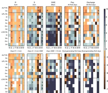
Figure 6. Comparison of the long-term trends (1950–2011) of the total equivalent precipitation depth, the snow water equivalent, the snowfall,
and the rainfall for the individual months November–May (N–M) and the winter season (W) for the alpine (ALP), upland (UPL) and lowland (LOW) sub-basins of the Rhine (Rh), Danube (Do), Elbe (El), Weser (We), Oder (Od), and Ems (Em). Trends are given as the yearly change relative to the mean of the period 1950–2011. Statistically significant trends atp <5 % are shown with a red star.
calculated for the individual months from November to May and for the sum over the entire winter season for all basins. In contrast to Fig. 5, the trends were calculated including years without RoS events and thus also account for changes in the frequency of occurrence. For R around 20 % of the trends were statistically significant, forS30 %, and for mean SWE 42 %. For the sample of all events, around 10 % of the trends inPeqand 17 % of the trends in discharge were
statis-tically significant atp <0.05, while for the selected poten-tially flood-generating events only around 2 % of the trends were statistically significant. Overall, the detected long-term trends range between −4 and+4 % for all variables.R in-creased in November, December, and April in the alpine sub-basins and from January to March in the upland and lowland sub-basins. In contrast,S showed overall decreasing trends. Similar toS, SWE decreased for all elevation ranges and all winter months, with especially large negative trends in April in some upland and all lowland basins. Similarly, the number of days with SWE>10 mm SWE decreased between Jan-uary and April in the upland and lowland sub-basins, espe-cially in April in the Ems and Weser sub-basins, indicating a shortening of the winter duration in these regions. No clear
trends in the number of days with SWE>10 mm SWE were identified in the alpine regions. In the alpine sub-basins, the trends inPeq were overall positive during the early winter
season and negative in April and May. In the upland sub-basins the trendsPeqwere positive in January and February
and negative from March to May. In the lowland sub-basins these trends were negative for all winter months. The trends inPeq for the selected RoS days were very similar to those
for all RoS days in the alpine and upland sub-basins, but the lowland trends differed with positive trends from November to January. The trends in corresponding peak discharges were very similar to the trends inPeq, with slightly more positive
values for the entire winter season for all basins and elevation ranges except for the Ems and Oder sub-basins, where trends were negative.
* * * * * * * * * * * * * * * * * * * * * * * * * * * * * * * * * * * * * * * * * * * * * * * * * * * * * * * * * * * * * * * * * * * * * * * * * * * * * * * * * * * * *
Sum Sum Mean All RoS days All RoS days
ALP Rh Do UPL Rh El We Do Em Od LOW Rh El We Em Od
Trend relative to mean (%)
−10 −8 −6 −4 −2 0 2 4 6 8 10 R S SWE Peq Discharge
Days R > 3 mm Days S > 0 mm SWE Days SWE > 10 mm flood-generating RoS days flood-generating RoS days
N D J F M A M W
N D J F M A M W
N D J F M A M W
N D J F M A M W
N D J F M A M W
N D J F M A M W
N D J F M A M W
N D J F M A M W
N D J F M A M W
N D J F M A M W
[image:11.612.113.482.64.381.2]ALP Rh Do UPL Rh El We Do Em Od LOW Rh El We Em Od * * * * * * * * * * * * * * * * * * * * * * * *
Figure 7. Comparison of the short-term trends (1990–2011) of the total equivalent precipitation depth, the snow water equivalent, the
snowfall, and the rainfall for the individual months November–May (N–M) and the winter season (W) for the alpine (ALP), upland (UPL) and lowland (LOW) sub-basins of the Rhine (Rh), Danube (Do), Elbe (El), Weser (We), Oder (Od), and Ems (Em). Trends are given as the yearly change relative to the mean of the period 1990–2011. Statistically significant trends atp <5 % are shown with a red star.
and May and negative in the rest of the winter for all basins. Also opposite to the long-term trends, short-term trends inS
were positive from November to March and negative in April in all upland and lowland sub-basins. The alpine sub-basins showed, in contrast, negative trends in S for the long-term and short-term periods. The same differences are reflected in SWE, with high positive short-term trends from December to March, only negative trends in May in the upland and low-land sub-basins, and negative trends for all winter months in the alpine sub-basins. Trends in thePeqof all RoS days
were negative in the alpine sub-basins for all winter months, but the trends in potentially flood-generating RoS days were mostly positive. In the upland and lowland sub-basins, trends were negative in November, December, and April and posi-tive from January to March, and a particularly strong increase in thePeqof the selected RoS days was observed from
Jan-uary to March. This increase was also reflected in the trends of the corresponding peak discharge in all upland and low-land sub-basins. In January and February, the trends in dis-charge had a similar direction to the trends in Peqbut were
smaller.
The sensitivity analysis of the base temperature showed that increasing or decreasingTbby±1◦C had little impact
on the direction of the trends. On average, 95 % of the cal-culated trends showed the same direction. ThePeqof the
se-lected potentially flood-generating RoS days was the most sensitive with still around 80 % of the trends having the same direction. Rainfall trends were the least sensitive, with 100 % showing the same direction. The calculated trends were also insensitive to the degree-day factorMfwhen testing values
ranging from 2 to 5 mm◦C−1day−1. This low sensitivity can be explained by the fact that the trend analysis considers the relative changes to the mean.
4 Discussion
widespread snow cover over the study area in the beginning of January, and its remarkable depth with extreme values at several locations in Germany (e.g. Böhm et al., 2011; Bastian et al., 2011; Karuse, 2011; LHW, 2011; Fell, 2011; Besler, 2011). The snowpack therefore represented a very large wa-ter reservoir available for runoff. On the other hand, the cli-matic conditions with thawing temperatures and rainfall in January provided the required energy to melt the snowpack. Runoff was therefore generated during a very short time, with a maximum of 6 days for each flood wave, and simul-taneously reached the upper and lower parts of the Rhine, Danube, Weser, Elbe, Oder, and Ems basins, thus causing floods in most areas. Even if most of these discharges corre-spond to return periods of less than 10 years and thus are not statistically extreme (Kohn et al., 2014), this RoS event em-phasises the large-scale impact of such events and their po-tential of shifting the annual peak flow from the late winter season to early winter season. This event therefore represents a good reference for the characterisation of RoS events with flood-generation potential.
The runoff generation from RoS events is influenced by many antecedent conditions and physical processes such as the thermal, mass, and wetness conditions of the snowpack, or the snow metamorphism, the water movement through the wet snow, the interaction of melt water with underly-ing soil, or the overland flow at the snow base (Sunderly-ingh et al., 1997; Marks et al., 1998). A physically based model would be needed to continuously simulate the development of the snowpack as well as evapotranspiration, sublimation, and in-filtration, and thus to estimate the actual runoff generation. In a large-scale analysis however, parameterisation for all pro-cesses would be difficult. The almost continental scale of the study requires considering data availability and conceptual-isation of processes dominant at that scale. In the case of this study, these are the hydrometeorological magnitude of rain-on-snow events and the temporal scale relevant to flood generation at the large scale. The aim of this study is there-fore not to improve the description or understanding of runoff generation at the hillslope or small catchment scale during a RoS event, but to analyse RoS events’ long-term evolution at the large scale. Therefore, no runoff is calculated, but the equivalent precipitation depth is related to the RoS event by its comparison to measured peak discharge during the event. However, even at the small catchment scale, Rössler et al. (2014) concluded that the hydrometeorological conditions are the main factors quantifying RoS-driven flood events.
Despite its apparent simplicity compared to energy bal-ance methods, Ohmura (2001) showed that the temperature-based melt index model was sufficiently accurate for most practical purposes, and was justified on physical grounds since the air temperature is the main heat source for the at-mospheric longwave radiation. This model has the advan-tage that it needs only daily precipitation and temperature data, often the only available data, and has already proved to be accurate enough for large-scale modelling if the
inten-tion is to identify basin-scale processes (Merz and Blöschl, 2003). The conceptual temperature index model employed in this study allowed estimating the potential snowpack and snowmelt. Even when the degree-day factor was generalised for the entire study area, the method led to a good estimation of the equivalent precipitation depth, was accurate enough to recognise known historical events, and was supported by the comparison to measured peak discharges during the RoS event. This validation of RoS events and the selection and analysis of potential flood-generating RoS events add to pre-vious studies, which have mostly looked only at RoS days.
Using the January 2011 RoS-driven flood events as a ref-erence, it was therefore possible to identify the magnitude of rainfall, the snowpack, and the percentage of snowmelt in the equivalent precipitation depth as the main characteristics of a RoS event and as the major characteristics for runoff gen-eration at the large scale. The resulting threshold values of 3 mm for rainfall, 10 mm SWE for snowpack, and 20 % for snowmelt content inPeqwere able to detect all documented
historical RoS-driven flood events in the time series and to specifically select only potentially flood-generating RoS events. These thresholds have therefore proved to be good indicators for RoS-driven flood events. The snowpack thresh-old (10 mm SWE) is not only representative for the event of January 2011, but also corresponds to the definition of the beginning of the winter by Beniston (2012) and Bavay et al. (2013). The advantage of the approach of identifying RoS events with threshold values is that it can easily be applied to other basins where discharge measurements are available, and it represents a useful tool for analysing changes in fre-quencies and magnitudes of those events.
The results showed an elevation dependence of RoS events in all basins, confirming the observations of different previ-ous studies (e.g. Merz and Blöschl, 2003; Pradhanang et al., 2013). RoS events generally have a high impact on discharge peaks in alpine and upland basins. These events are most likely to lead to high discharges (quantiles of 0.7–1 in the alpine sub-basins and even 0.8–1 in the upland sub-basins), and they therefore have a real potential for generating floods in these regions. This result is in agreement with the ob-servation of Sui and Koehler (2001) that RoS events play a more important role in runoff generation than pure rainfall events for topographical elevations above about 400 m a.s.l.
the very wet autumn 2010, which led to already very high water levels and discharges at the beginning of January (e.g. Kohn et al., 2014).
One challenge in the trend analysis of extreme RoS events is the censored data; i.e. events do not occur every year. Most methods for trend analysis try to statistically disclose out-liers, as for example the Sen slope method. In our case, how-ever, the outliers are often exactly the values that need to be considered. Therefore, linear regression was found to be the method better suited for the trend analysis. The zeros also ex-plain why many trends were not statistically significant. This is a well-known problem in hydrology. Kundzewicz et al. (2012) observed for example that the strong natural variabil-ity of hydrologic events can alter trend detection, and IPCC (2012) pointed out that, due to the fact that extreme events are per definition rare, long record lengths are required to al-low for detection of trends in extremes. However, the lack of statistical significance does not mean that the trends do not exist, but that the hypothesis of no existing trends could not be rejected. As discussed, e.g., by Stahl et al. (2010) in more detail, the application of trend tests has been criticised ex-tensively in the literature because many assumptions are not met by hydrological time series data. As suggested in other large-scale studies, a systematic regional consistency of trend direction and magnitude is therefore a more relevant result than the number of statistical significances. In this study, the value of the trend analysis has its main value not in the abso-lute numbers estimated but in the comparison of the consis-tency in the trends of the individual components involved in rain-on-snow events.
The estimated magnitudes and frequencies revealed a dif-ferent importance of RoS events in the difdif-ferent elevation zones represented by the sub-basins. Nearly half of the to-tal winter precipitation (rain and snow) and even two-thirds of the late winter precipitation contribute to RoS events in the alpine sub-basins, while this contribution is one-third in the upland basins, and only one-fifth in the lowland sub-basins. The largest changes in frequencies were observed in the upland basins, where late winter RoS events have be-come less frequent since the 1990s. This change in frequen-cies can be explained by the decreasing trends in snow depth observed in the late winter season in these areas (Figs. 6 and 7) and therefore by a decreasing probability of rain falling on a snow cover in the late winter season. In contrast, the trends in rainfall are positive in the early winter season, increas-ing the probability for RoS events, especially in January and February. These results agree well with the observations of many studies worldwide (e.g. Birsan et al., 2005; Knowles et al., 2006; Ye, 2008; Ye et al., 2008). Trends in magni-tude vary from one basin to another. The upland Elbe and Rhine sub-basins show positive trends in the early and late winter seasons, while the other upland sub-basins have nega-tive trends. This difference can be explained by the more fre-quent and stable snow cover in the upland basins of the Elbe and Rhine. The corresponding positive trends in the
mea-sured discharges of RoS events were positive from January to March in the alpine and upland sub-basins, and especially in March for the short-term trend analysis, suggesting an im-pact of this increasing magnitude.
Trends have to be interpreted carefully since they depend on the choice of the time period, which can be influenced by many climatic factors and also by extreme values. The anal-ysis of long-term (1950–2011) vs. short-term (1990–2011) trends showed different, even opposite, results for all vari-ables. Overall, long-term trends are smaller than short-term trends. The greatest difference between both periods is in the trend in the mean SWE. In the long-term analysis, snowpack has declined in all basins, while it has increased in the short-term period in all basins except the alpine sub-basins. Fricke (2006) observed that the average snowpack in Germany for the period 1961–1990 was substantially higher than for the period 1991–2000. The 21st century was characterised by extreme events. The winter 2005–2006 and December 2010, for example, were identified as extremely snow rich in Ger-many (Fricke, 2006; Pinto et al., 2007; Böhm et al., 2011). This explains the differences in the trends, since the extreme events of the 21st century will have more weight in a shorter time series, especially if they occurred in the beginning of the period such as for the lower observed snow depth.
The alpine sub-basins show different trends to the upland and lowland basins. While the upland and lowland sub-basins have negative trends in the long-term analysis and pos-itive trends in the short-term analysis, SWE in the alpine sub-basins decreased in both the long- and short-term trend anal-yses. This difference can be explained by the climatic condi-tions specific to the alpine regions, which are very different to those in the upland and lowland sub-basins. For example, while exceptionally great SWE was measured all over Ger-many in December 2010, the Swiss Alps experienced snow-packs below average (e.g. Trachte et al., 2012; Techel and Pielmeier, 2013). In another study in the Swiss Alps, Benis-ton (2012) found that the wintertime precipitation declined between 15 and 25 % over the 1931–2010 period and that the number of snow-sparse winters has increased in the last 40 years, while the number of snow-abundant winters has de-clined. But in the meantime, some winters since the 1990s have experienced record-breaking snow amounts and dura-tions (Beniston, 2012). Rainfall also shows opposite trends, increasing for the long time series and mostly decreasing for the short time series in the wintertime. As snowpack and rain-fall both influence the occurrence of RoS events, trends in RoS days are therefore difficult to identify for the long-term analysis, since rainfall is increasing but snow depth is de-creasing.
potentially flood-generating RoS days are even more posi-tive, leading to the conclusion that they have become an im-portant factor for the winter discharge and that the occurrence of maximum peak flow from RoS events between January and March has become more frequent since the 1990s.
5 Conclusions
In a context of climate change, snowpack and precipitation in the wintertime are very likely to change and therefore may influence the frequency and magnitude of the flood haz-ard from rain-on-snow events in central Europe. The anal-ysis of causes and trends for past RoS events is challeng-ing since these events depend on many influences. Definchalleng-ing threshold values to characterise RoS events allowed identify-ing the events with potentially high impact on river discharge on a large scale and analysing them for trends in frequency and magnitude. The results showed an elevation dependence of RoS events and suggest they have the strongest impacts in upland regions, where an increasing magnitude of these events was observed. However, the frequency of RoS events decreased in the second half of the time period 1950–2011 in the late winter season in upland and lowland basins and can be related to decreasing trends in snowpack in the late winter season. Increasing trends in rainfall in the early winter season as well as increasing trends in equivalent precipitation depth during RoS events in some upland sub-basins suggest that these events have become more important at this elevation class.
The results show the importance of the choice of the anal-ysed period for the detection of trends, with opposite trends found for snow water equivalent in the long-term and short-term periods. The 21st century has been affected by several extreme events, which makes the analysis even more diffi-cult. As the example of January 2011 in Germany and cen-tral Europe showed, rain can release a large amount of wa-ter stored in the snowpack and RoS events can cause very widespread flood events, delivering a large amount of water to the streams within a very short time. If such events are likely to become more frequent in the future in certain basins and elevation ranges, the winter flood hazard will increase. Therefore, there is a real need for an improved understanding of the relation between RoS events and flooding, and more analysis is needed on their occurrence at different scales.
Acknowledgements. In part, the study was funded by the Bun-desanstalt für Gewässerkunde as part of a reanalysis of the hydrological extremes during the year 2011. The article processing charge was funded by the German Research Foundation (DFG) and the Albert Ludwig University Freiburg in the funding pro-gramme Open Access Publishing. The authors thank J. U. Belz for his support with data and advice. The authors would also like to acknowledge the E-OBS data set from the EU-FP6 project ENSEMBLES (http://ensembles-eu.metoffice.com) and the data
providers ECA&D project (http://www.ecad.eu) for providing precipitation and temperature data. The authors also thank the environmental agencies of the German federal states for providing discharge data. Finally, the authors acknowledge two anonymous reviewers for their thoughtful comments that helped improve the manuscript.
Edited by: G. Di Baldassarre
References
Bastian, D., Göbel, K., Klump, W., Kremer, M., Lipski, P., and Löns-Hanna, C.: Das Januar-Hochwasser 2011 in Hessen, Hy-drologie in Hessen, Heft 6, Hessische Landesamt für Umwelt und Geologie, Wiesbach, Germany, 2011 (in German).
Bavay, M., Grünewald, T., and Lehning, M.: Response of snow cover and runoff to climate change in high Alpine catchments of Eastern Switzerland, Adv. Water Resour., 55, 4–16, 2013. Beniston, M.: Is snow in the Alps receding or disappearing?, WIREs
Clim. Change, 3, 349–358, doi:10.1003/wcc.179, 2012. Besler, C.: Dokumentation Elbehochwasser Januar 2011, Teil 1:
Meteorologische Situation und hydrologischer Verlauf des Hochwassers, Report, Staatliches Amt für Landwirtschaft und Umwelt (StALU) Westmecklenburg, Schwerin, Germany, 2011 (in German).
Birsan, M.-V., Molnar, P., Burlando, P., and Pfaundler, M.: Stream-flow trends in Switzerland, J. Hydrol., 314, 312–329, 2005. Blöschl, G., Kirnbauer, R., and Gutknecht, D.: Modelling snowmelt
in a mountainous river basin on an event basis, J. Hydrol., 113, 207–229, 1990.
Böhm, U., Fiedler, A., Machui-Schwanitz, G., Reich, T., and Schneider, G.: Hydrometeorolgische Analyse der Schnee- und Tauwettersituation im Dezember 2010/Januar 2011 in Deutsch-land, Report, Deutscher Wetterdienst (DWD), Offenbach, Ger-many, 2011 (in German).
Collins, E. H.: Relationship of degree-days above freezing to runoff, EOS T. Am. Geophys. Un., 15, 624–629, 1934.
Corps of Engineers: Summary report of the snow investigations, snow hydrology, US Army Engineer Division (North Pacific, 210 Custom House, Portland, Oregon), 437 pp., 1956.
Fell, E.: Kurzbericht: Hochwasser im Rheingebiet – Januar 2011, Report, Landesamt für Umwelt Wasserwirtschaft und Gewer-beaufsicht (LUWG) Rheinland-Pfalz, Mainz, Germany, 2011 (in German).
Finsterwalder, S. and Schunk, H.: Der Suldenferner, Zeitschrift des Deutschen und Oesterreichischen Alpenvereins, 18, 72–89, 1887 (in German).
Floyd, W. and Weiler, M.: Measuring snow accumulation and abla-tion dynamics during rain-on-snow events: innovative measure-ment techniques, Hydrol. Process., 22, 4805–4812, 2008. Fricke, W.: Wieder mehr Schnee im Winter?, Global Atmosphere
Watch, Brief 33, Deutscher Wetterdienst (DWD), Germany, March 2006 (in German).
Haylock, M. R., Hofstra, N., Klein Tank, A. M. G., Klok, E. J., Jones, P. D., and New, M.: A European daily high-resolution gridded dataset of surface temperature and pre-cipitation for 1950–2006, J. Geophys. Res., 113, D20119, doi:10.1029/2008JD10201, 2008.
Hock, R.: Temperature index melt modeling in mountain areas, J. Hydrol., 282, 104–115, 2003.
IPCC: Summary for policymakers, in: Managing the risks of ex-treme events and disasters to advance climate change adaptation. A special report of working groups I and II of the Intergovern-mental Panel on Climate Change IPCC, Cambridge University Press, Cambridge, UK and New York, NY, USA, 3–21, 2012. Karuse, P.: Gewässerkundlicher Monatsbericht Januar 2011,
Re-port, Bayerisches Landesamt für Umwelt und Geologie (HLUG), Wiesbaden, Germany, 2011 (in German).
Kattelmann, R. C.: Macropores in snowpacks of Sierra Nevada, Ann Glaciol, 6, 272–273, 1985.
Kattelmann, R. C.: Flooding from rain-on-snow events in the Sierra Nevada, in: Destructive water: Water-caused natural disasters, their abatement and control, edited by: Leavesley, G. H., Pro-ceedings of the conference, Anaheim, California, June 1996, IAHS Publication, 239, 59–65, 1997.
Knowles, N., Dettinger, M. D., and Cayan, D. R.: Trends in snowfall versus rainfall in the Western United States, J. Climate, 19, 4545– 4559, 2006.
Kohn, I., Freudiger, D., Rosin, K., Stahl, K., Weiler, M., and Belz, J.: Das hydrologische Extremjahr 2011: Dokumentation, Einordnung, Ursachen und Zusammenhänge, Report, Mitteillung Nr. 29, Bundesanstalt für Gewässerkunde (Hrsg.), Koblenz, Ger-many, 2014 (in German).
Köplin, N., Schädler, B., Viviroli, D., and Weingartner, R.: Season-ality and magnitude of floods in Switzerland under future climate change, Hydrol. Process., 28, 2567–2578, doi:10.1002/hyp.9757, 2014.
Kundzewicz, Z. W., Plate, E. J., Rodda, H. J. E., Rodda, J. C., Schnellnhuber, H. J., and Strupczewski, W. G.: Changes in flood risk – setting the stage, in: Changes in Flood Risk in Europe, edited by: Kundzewicz, Z. W., IAHS Press, Wallingford, 11–26, 2012.
Lefebvre, C. and Becker, A.: Das Klima des Jahres 2011 im glob-alen Massstab, Klimastatusbericht, Report, Deutscher Wetterdi-enst (DWD), Offenbach, Germany, 2011 (in German).
LHW: Bericht über das Hochwasser Januar 2011, Report, Lan-desbetrieb für Hochwasserschutz und Wasserwirtschaft (LHW) Sachsen-Anhalt, Magdeburg, Germany, 2011 (in German). Mann, H. B.: Nonparametric test against trend, Econometrica, 13,
245–259, 1945.
Marks, D., Kimball, J., Tingey, D., and Link, T.: The sensitivity of snowmelt processes to climate conditions and forest cover during rain-on-snow: a case study of the 1996 Pacific Northwest flood, Hydrol. Process., 12, 1559–1587, 1998.
Martinec, J. and Rango, A.: Parameter values for snowmelt runoff modelling, J. Hydrol., 84, 197–219, 1986.
McCabe, G. J., Clark, M. P., and Hay, L. E.: Rain-on-snow events in the western United States, B. Am. Meteorol. Soc., 88, 319–328, doi:10.1175/BAMS-88-3-319, 2007.
Merz, R. and Blöschl, G.: A process typology of regional floods, Water Resour. Res., 39, 1340, doi:10.1029/2002WR001952, 2003.
Nied, M., Hundecha, Y., and Merz, B.: Flood-initiating catchment conditions: a spatio-temporal analysis of large-scale soil mois-ture patterns in the Elbe River basin, Hydrol. Earth Syst. Sci., 17, 1401–1414, doi:10.5194/hess-17-1401-2013, 2013. Ohmura, A.: Physical basis for the temperature-based melt-index
method, J. Appl. Meteorol., 40, 753–761, 2001.
Pinto, J. G., Brücher, T., Fink, A. H., and Krüger, A.: Extraordinary snow accumulations over parts of central Europe during winter of 2005/06 and weather-related hazards, Weather, 62, 16–21, 2007. Pradhanang, S. M., Frei, A., Zion, M., Schneiderman, E. M., Steen-huis, T. S., and Pierson, D.: Rain-on-snow events in New York, Hydrol. Process., 27, 3035–3049, 2013.
Renard, B., Lang, M., Bois, P., Dupeyrat, A., Mestre, O., Niel, H., Sauquet, E., Prudhomme, C., Parey, S., Paquet, E., Neppel, L., and Gaillhard, J.: Regional methods for trend detection: Assess-ing field significance and regional consistency, Water Resour. Res., 44, W08419, doi:10.1029/2007WR006268, 2008. Rössler, O., Froidevaux, P., Börst, U., Rickli, R., Martius, O., and
Weingartner, R.: Retrospective analysis of a nonforecasted rain-on-snow flood in the Alps – a matter of model limitations or unpredictable nature?, Hydrol. Earth Syst. Sci., 18, 2265–2285, doi:10.5194/hess-18-2265-2014, 2014.
Singh, P., Spitzbart, G., Hübl, H., and Weinmeinster, H. W.: Hydro-logical response of snowpack under rain-on-snow events: a field study, J. Hydrol., 202, 1–20, 1997.
Stahl, K., Hisdal, H., Hannaford, J., Tallaksen, L. M., van Lanen, H. A. J., Sauquet, E., Demuth, S., Fendekova, M., and Jódar, J.: Streamflow trends in Europe: evidence from a dataset of near-natural catchments, Hydrol. Earth Syst. Sci., 14, 2367–2382, doi:10.5194/hess-14-2367-2010, 2010.
Sui, J. and Koehler, G.: Rain-on-snow induced flood events in Southern Germany, J. Hydrol., 252, 205–220, 2001.
Surfleet, C. G. and Tullos, D.: Variability in effect of climate change on rain-on-snow peak flow events in temperate climate, J. Hy-drol., 479, 24–34, 2013.
Techel, F. and Pielmeier, C.: Schnee und Lawinen in den Schweizer Alpen, Hydrologisches Jahr 2010/11, Report, WSL-Institut für Schnee- und Lawinenforschung SLF, Davos, Switzerland, 2013 (in German).
Trachte, K., Obregón, A., Bissolli, P., Kennedy, J. J., Parker, D. E., Trigo, R. M., Barriopedro, D., Kendon, M., Prior, J., Achberger, C., Gouvela, C., Sensoy, S., Hovsepyan, A., and Grigoryan, V.: State of the Climate in 2011, Regional Climates – Europe, B. Am. Meteorol. Soc., 93, 186–199, 2012.
Venables, W. N. and Ripley, B. D.: Modern Applied Statistics Using S, 4th Edn., Springer, New York, United States, 2002.
Wetterchronik: http://www.wetterzentrale.de/cgi-bin/ wetterchronik/home.pl, access: 14 June 2013, 2001.