www.hydrol-earth-syst-sci.net/18/287/2014/ doi:10.5194/hess-18-287-2014
© Author(s) 2014. CC Attribution 3.0 License.
Hydrology and
Earth System
Sciences
Linking the river to the estuary: influence of river discharge on tidal
damping
H. Cai1, H. H. G. Savenije1, and M. Toffolon2
1Department of Water Management, Faculty of Civil Engineering and Geosciences, Delft University of Technology, Stevinweg 1, P.O. Box 5048, 2600 GA Delft, the Netherlands
2Department of Civil, Environmental and Mechanical Engineering, University of Trento, Trento, Italy
Correspondence to: H. Cai ([email protected])
Received: 26 June 2013 – Published in Hydrol. Earth Syst. Sci. Discuss.: 15 July 2013 Revised: 12 December 2013 – Accepted: 15 December 2013 – Published: 22 January 2014
Abstract. The effect of river discharge on tidal damping in estuaries is explored within one consistent theoretical frame-work where analytical solutions are obtained by solving four implicit equations, i.e. the phase lag, the scaling, the damp-ing and the celerity equation. In this approach the dampdamp-ing equation is obtained by subtracting the envelope curves of high water and low water occurrence, taking into account that the flow velocity consists of a tidal and river discharge component. Different approximations of the friction term are considered in deriving the damping equation, resulting in as many analytical solutions. In this framework it is possible to show that river discharge affects tidal damping primarily through the friction term. It appears that the residual slope, due to nonlinear friction, can have a substantial influence on tidal wave propagation when including the effect of river dis-charge. An iterative analytical method is proposed to include this effect, which significantly improved model performance in the upper reaches of an estuary. The application to the Modaomen and Yangtze estuaries demonstrates that the pro-posed analytical model is able to describe the main tidal dy-namics with realistic roughness values in the upper part of the estuary where the ratio of river flow to tidal flow amplitude is substantial, while a model with negligible river discharge can be made to fit observations only with unrealistically high roughness values.
1 Introduction
[image:2.595.102.495.61.220.2]
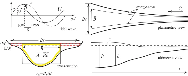
Fig. 1. Sketch of the estuary geometry and basic notations (after Savenije et al., 2008).
The treatment of the nonlinear friction term is key to find-ing an analytical solution for tidal hydrodynamics. The non-linearity of the friction term has two sources: the quadratic stream velocity in the numerator and the variable hydraulic radius in the denominator (Parker, 1991). The classical lin-earization of the friction term was first obtained by Lorentz (1926) who, disregarding the variable depth, equated the dis-sipation by the linear friction over the tidal cycle to that of the quadratic friction. An extension to include river dis-charge was provided by Dronkers (1964). In this seminal work, he derived a higher-order formulation using Cheby-shev polynomials, both with and without river discharge, re-sulting in a close correspondence with the quadratic velocity. Godin (1991, 1999) showed that quadratic velocity can be well approximated by using only the first- and third-order terms of the non-dimensional velocity. However, none of the above linearizations took into account the effect of the peri-odic variation of the hydraulic radius (to the power 4/3 in the Manning–Strickler formulation) in the denominator of the friction term. On the other hand, Savenije (1998), using the envelope method (see Appendix A), obtained a damping equation that takes account of both the quadratic velocity and the time-variable hydraulic radius in the denominator.
This paper builds on a variety of previous publications on analytical approaches to tidal wave propagation and damp-ing. A first attempt to include the effect of river discharge by Horrevoets et al. (2004) used the quasi-nonlinear method of Savenije (2001), assuming constant velocity amplitude, wave celerity and phase lag. Cai et al. (2012b) applied this model to the Modaomen estuary. In the present paper we make use of the analytical framework for tidal wave prop-agation by Cai et al. (2012a), but including for the first time the effect of river discharge in a hybrid model that performs better. Moreover, fully analytical equations accounting for four spatial variables (velocity amplitude, tidal amplitude, wave celerity and phase lag) of tidal propagation are now pre-sented, demonstrating that the effect of river discharge is sim-ilar to that of friction. In addition, building on the research
by Vignoli et al. (2003) on nonlinear frictional residual ef-fects on tidal propagation, the influence of residual slope on tidal wave propagation has been taken into account, which significantly improved performance, especially in the up-stream part of estuaries where the effect of river discharge is considerable.
In the following section, we introduce the relevant dimen-sionless parameters that control tidal hydrodynamics. The analytical framework for tidal wave propagation is summa-rized in Sect. 3. The damping equations that take account of river discharge are presented in Sect. 4 and the method to in-clude the residual slope in the analytical solution is reported in Sect. 5. Section 6 presents a comparison of the different analytical approaches and a sensitivity analysis. The model is subsequently compared against the fully nonlinear numer-ical results and applied to two real estuaries where the effect of the river discharge is apparent in the upstream part of the estuary. The paper closes off with conclusions in Sect. 7.
2 Formulation of the problem
We consider a tidal channel with varying width and depth, a mostly rectangular cross section and lateral storage areas described by the storage width ratiorS=BS/B, which is the ratio between the storage widthBS and the average stream widthB (hereafter overbars denote tidal averages). The ge-ometry of the idealized tidal channel is described in Fig. 1, together with a simplified picture of the periodic oscillations of water level and velocity defining the phase lag. It is gen-erally accepted that the main geometric parameters of allu-vial estuaries (tidally averaged cross-sectional area, width and depth) can be well described by exponential functions (e.g. Savenije, 1992):
A=A0exp
−x
a
, B=B0exp
−x
b
, h=h0exp
−x
d
,(1) where x is the longitudinal coordinate directed landward,
Table 1. The definition of dimensionless parameters.
Dimensionless parameters
Independent Dependent
Damping number δ=c0dζ /(ζ ωdx) Tidal amplitude at the downstream boundary Velocity number
ζ0=η0/h µ=υ/ (rSζ c0)=υ h/ (rSη c0) Estuary shape number Celerity number
γ=c0/(ω a) λ=c0/c
Reference friction number Phase lag
χ0=rSg c0/
K2ω h4/3
ε=π/2−(φz−φU)
Tidal amplitude ζ=η/h Friction number
χ=χ0ζ
h
1−(4ζ /3)2i−1=rSf c0ζ / ω h
flow depth,a,b,d are the convergence length of the cross-sectional area, width, and depth, respectively, and the sub-script 0 relates to the reference point near the estuary mouth. It follows fromA=B hthata=b d/(b+d).
The one-dimensional hydrodynamic equations in an allu-vial estuary are given by (e.g. Savenije, 2005, 2012)
∂U ∂t +U
∂U ∂x +g
∂h
∂x +g Ib+g F + g h
2ρ ∂ρ
∂x =0, (2) rs
∂h ∂t +U
∂h ∂x +h
∂U ∂x +
h U
B ∂B
∂x =0, (3)
wheretis the time,Uis the cross-sectional average flow ve-locity,his the flow depth,gis the gravitational acceleration,
Ib is the bottom slope,ρ is the water density andF is the friction term, defined as
F = U|U|
K2h4/3, (4)
whereKis the Manning–Strickler friction coefficient. If we define the water level variationz=h−h, then for a small tidal amplitude to depth ratio, we find
U∂h ∂x =U
∂ z+h
∂x =U
∂z ∂x +
h U
h ∂h ∂x ≈U
∂z ∂x +
h U
h ∂h ∂x.(5) Substituting Eq. (5) into Eq. (3) and making use of Eq. (1), the following equation is obtained:
rS
∂z ∂t +U
∂z ∂x +h
∂U ∂x −
h U
a =0, (6)
which has the advantage that the depth convergence is im-plicitly taken into account by the convergence of the tidally averaged cross-sectional area.
The system is forced by a harmonic tidal wave with a tidal periodT and a frequencyω= 2π/T at the mouth of the es-tuary. As schematically shown in Fig. 1, the amplitudes of
the tidal water levelzand velocityUare represented by the variables ofηandυ, respectively. The phases of the water level and velocity oscillations are indicated byφz andφU,
respectively. In a Lagrangean approach, we assume that the water particle moves according to a simple harmonic wave and the influence of river discharge on tidal velocities is not negligible. As a result, the instantaneous flow velocityV for a moving particle is made up of a steady componentUr, cre-ated by the discharge of freshwater, and a time-dependent componentUt, contributed by the tide:
V =Ut−Ur, Ut =υsin(ω t ), Ur =Qf/A, (7) whereQf is the freshwater discharge, directed against the positivex-direction.
It can be shown that the estuarine hydrodynamics is con-trolled by three dimensionless parameters in the case of neg-ligible river discharge (Toffolon et al., 2006; Savenije et al., 2008; Toffolon and Savenije, 2011; Cai et al., 2012a). Table 1 presents these independent dimensionless parameters that depend on the geometry and external forcing. They are:ζ0 the dimensionless tidal amplitude at the downstream bound-ary,γ the estuary shape number (representing the effect of cross-sectional area convergence and depth), andχ0the ref-erence friction number (describing the frictional dissipation). These parameters containc0, representing the classical wave celerity of a frictionless progressive wave in a constant-width channel:
c0=
q
g h/rS. (8)
The six dependent dimensionless variables are also presented in Table 1. They are:δ the damping number (a dimension-less description of the rate of increase,δ >0, or decrease,
Table 2. Analytical framework for tidal wave propagation (Cai et al., 2012a).
Case Phase lag tan(ε) Scalingµ Celerityλ2 Dampingδ
General
Quasi-nonlinear
λ/(γ−δ) cos(ε)/(γ−δ) 1−δ(γ −δ)
γ /2−χ µ2/2
Linear γ /2−4χ µ/(3π λ)
Dronkers γ /2−8χ µ/(15π λ)−16χ µ3λ/(15π )
Hybrid γ /2−4χ µ2/(9π λ)−χ µ2/3
Constant cross-section
Quasi-nonlinear
−λ/δ −cos(ε)/δ 1+δ2
−χ µ2/2
Linear −4χ µ/(3π λ)
Dronkers −8χ µ/(15π λ)−16χ µ3λ/(15π )
Hybrid −4χ µ2/(9π λ)−χ µ2/3
Frictionless (γ <2) p4/γ2−1 1 1−γ2/4 γ /2
Frictionless (γ≥2) 0
γ−pγ2−4
/2 0
γ −pγ2−4
/2
Ideal estuary 1/γ
q
1/ 1+γ2
1 0
ratio between the theoretical frictionless celerity in a pris-matic channel and the actual wave celerity),εthe phase lag between high water (HW) and high water slack (HWS) or between low water (LW) and low water slack (LWS),ζ the dimensionless tidal amplitude that varies along the estuary, and finallyχthe friction number as a function ofζ (Toffolon et al., 2006; Savenije et al., 2008). The friction number con-tainsf as the dimensionless friction factor resulting from the envelope method (Savenije, 1998):
f = g
K2h1/3
h
1−(4ζ /3)2i −1
, (9)
where the factor 4/3 stems from a Taylor approximation of the exponent of the hydraulic radius in the friction term.
3 Analytical framework for tidal wave propagation with no river discharge
For negligible river discharge, the analytical solution of the one-dimensional hydrodynamic equations is obtained by solving four implicit equations, i.e. the phase lag, the scaling, the celerity and the damping equation (Savenije et al., 2008). The phase lag and scaling equations were derived from the mass balance equation by Savenije (1992, 1993) using a La-grangean approach. The celerity equation was developed by Savenije and Veling (2005) using a method of characteristics. The damping equation can be obtained through various meth-ods. Savenije (1998, 2001) introduced the envelope method that retains the nonlinear friction term, by subtracting the en-velopes at HW and LW.
Cai et al. (2012a) showed that different friction formu-lations can be used in the envelope method to arrive at an equal number of damping equations. In general, the main classes of the solutions are: (1) quasi-nonlinear so-lution with nonlinear friction term (Savenije et al., 2008); (2) linear solution with Lorentz’s linearization (Lorentz, 1926); (3) Dronkers’ solution with higher-order formulation
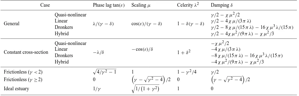
for quadratic velocity (Dronkers, 1964); (4) hybrid solu-tion characterized by a weighted average of Lorentz’s lin-earization, with weight 1/3, and the nonlinear friction term, with weight 2/3 (Cai et al., 2012a). In Table 2, we present the solutions of these four classes for the general case and for some particular cases, including constant cross-section (γ= 0), frictionless channel (χ= 0, both with subcritical con-vergence (γ <2) and supercritical convergence (γ≥2)) and ideal estuary (δ= 0). It was shown by Cai et al. (2012a) that the hybrid model provides the best predictions when com-pared with numerical solutions. Figure 2 shows the main de-pendent dimensionless parameters as function of the shape numberγ and the friction numberχ, obtained with the hy-brid model.
4 New damping equations accounting for the effect of river discharge
In the following, we extend the validity of the damping equa-tions by introducing the effect of river discharge into the dif-ferent approximations of the friction term. The dimension-less river dischargeϕis defined as
ϕ = Ur
υ . (10)
We show the procedure for including the effect of river dis-charge within the envelope method in Appendix A.
For a more concise notation, we refer to a general formu-lation of the damping parameter of the form:
δ = µ 2
1+µ2β (γ θ−χ µ λ 0) , (11) where we introduce the dimensionless parametersβ,θ, and
0 1 2 3 4 5 −3
−2 −1 0 1
Damping number
δ
0 1 2 3 4 5
0 0.2 0.4 0.6 0.8 1
Velocity number
μ
0 1 2 3 4 5
0 0.5 1 1.5 2 2.5
Shape number γ
Celerity number
λ
0 1 2 3 4 5
0 20 40 60 80 100
Shape number γ
Phase lag
ε
(
°
)
χ=0 (γ<2)
χ=0 (γ≥2)
χ=1
χ=2
χ=5
χ=10
χ=25
χ=50 Ideal a)
c)
b)
[image:5.595.131.468.66.316.2]d)
Fig. 2. Variation of damping numberδ, the velocity numberµ, celerity numberλand phase lagεwith the estuary shape numberγ for different values of the friction numberχ, obtained with the hybrid model. The green symbols represent the ideal estuary (see Table 2).
β =θ−rSζ
ϕ
µ λ. (12)
The correction factor θ accounts for the wave celerity not being equal at HW and LW, which depends onϕby
θ =1−p1+ζ −1 ϕ
µ λ. (13)
This parameter has a value smaller than unity, but is close to unity as long asζ1 althoughµ λ= sin(ε)is also less than 1. In practical applications, we can typically assume
θ≈1, but this is not a necessary assumption in our method. Finally, the parameter0depends on the specific approach, as it is discussed in the next sections.
4.1 The quasi-nonlinear approach
Savenije et al. (2008) presented a fully analytical solution for tidal wave propagation without linearizing the friction term through the envelope method. The method was termed quasi-nonlinear because it still made use of a regular har-monic function to describe the flow velocity. Horrevoets et al. (2004) introduced the effect of river discharge in the quasi-nonlinear model. Using the dimensionless parameters pre-sented in Table 1, Cai et al. (2012b) developed this solution into a general expression for tidal damping, where two zones are distinguished depending on the value of ϕ defined by Eq. (10).
In the tide-dominated zone, whereϕ < µ λ, the parameter
0introduced in Eq. (11) reads
0=µ λ "
1+ 8 3ζ
ϕ µ λ +
ϕ
µ λ 2#
, (14)
while in the river discharge-dominated zone, whereϕ≥µ λ, it becomes
0=µ λ "
4 3ζ +2
ϕ µ λ +
4 3ζ
ϕ
µ λ 2#
. (15)
4.2 Lorentz’s approach
The Fourier expansion of the productU|U| in the friction term is (Dronkers, 1964, 272–275)
U|U| = 1 4L0υ
2+1
2L1υ Ut, (16)
where the expressions of coefficients L0 and L1 when 0< ϕ <1 are
L0 = [2+cos(2α)]
2−4α
π
+ 6
π sin(2α), (17) L1 =
6
π sin(α)+
2
3π sin(3α)+
4−8α
π
cos(α), (18) with
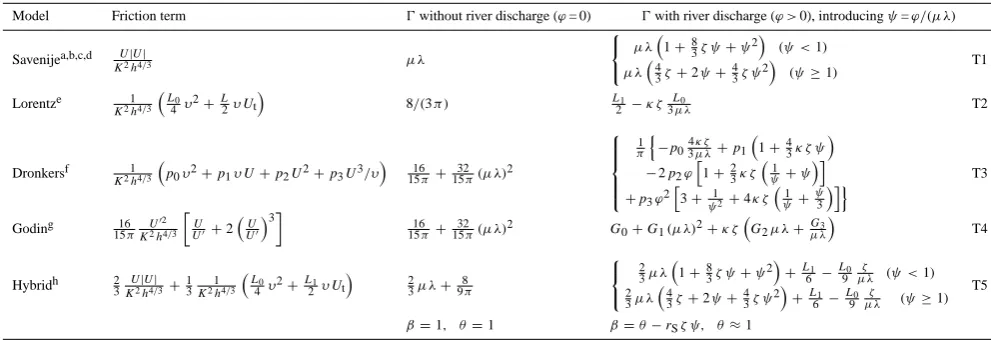
Table 3. Comparison of the terms in the damping Eq. (11) for different analytical methods. The effect of the time-dependent depth in the friction term for Lorentz’s, Dronkers’ and Godin’s method is accounted for by settingκ= 1 in the expressions for0, whereasκ= 0 describes the time-independent case.
Model Friction term 0without river discharge (ϕ= 0) 0with river discharge (ϕ >0), introducingψ=ϕ/(µ λ)
Savenijea,b,c,d U|U|
K2h4/3 µ λ
µ λ1+8
3ζ ψ+ψ2
(ψ <1)
µ λ43ζ+2ψ+4
3ζ ψ2
(ψ≥1) T1
Lorentze 1
K2h4/3
L
0
4 υ2+L2υ Ut
8/(3π ) L1
2 −κ ζ
L0
3µ λ T2
Dronkersf 1
K2h4/3
p0υ2+p1υ U+p2U2+p3U3/υ
16
15π +
32 15π(µ λ)2
1 π n
−p034κ ζµ λ+p1
1+4 3κ ζ ψ
−2p2ϕh1+2
3κ ζ
1
ψ +ψ
i
+p3ϕ2h3+ 1
ψ2+4κ ζ
1 ψ+ ψ 3 io T3
Goding 1516π U02
K2h4/3
U
U0+2
U U0
3
16
15π +1532π(µ λ)2 G0+G1(µ λ)2+κ ζ
G2µ λ+Gµ λ3
T4
Hybridh 2 3
U|U|
K2h4/3+ 1 3
1
K2h4/3
L
0
4 υ2+
L1
2 υ Ut
2
3µ λ+
8 9π 2
3µ λ
1+8
3ζ ψ+ψ2
+L1
6 −
L0 9
ζ
µ λ (ψ <1)
2
3µ λ
4
3ζ+2ψ+43ζ ψ2
+L1
6 −
L0 9
ζ
µ λ (ψ≥1)
T5
β=1, θ=1 β=θ−rSζ ψ, θ≈1
aSavenije (1998);bHorrevoets et al. (2004);cSavenije et al. (2008);dCai et al. (2012b);eLorentz (1926);fDronkers (1964);gGodin (1991, 1999);hCai et al. (2012a)
whereπ/2< α < πbecauseϕis positive. In caseϕ≥1,
L0= −2−4ϕ2, L1=4ϕ, (20) while the case ofϕ= 1 (i.e.Ur=υ) corresponds withα=π and leads toL0=−6 andL1= 4.
As a result, the development of the Lorentz’s friction term accounting for the effect of river discharge reads
FL = 1
K2h4/3
1
4L0υ 2+ 1
2L1υ Ut
, (21)
where the subscript L stands for Lorentz.
If the river discharge is negligible, i.e.Ur= 0 andα=π/2, Eq. (21) reduces to the classical Lorentz linearization and henceL0= 0 andL1= 16/(3π):
FL = 8 3π
υ
K2h4/3
Ut. (22)
With the envelope method, making use of friction term Eq. (21), it is possible to derive the parameter0in the damp-ing Eq. (11) (see Appendix A):
0L =
L1
2 . (23)
Extending Lorentz’s solution with the periodic variation of the depth in the denominator of the friction term (i.e. K2h4/3) is also possible. The resulting expression is reported in Table 3, whereκ=1 yields the time-dependent case, while Eq. (20) is recovered by settingκ= 0.
We also tested higher-order formulations of the friction term, such as proposed by Dronkers (1964) and Godin (1991, 1999), which we implemented in the envelope method arriv-ing at tidal damparriv-ing equations accountarriv-ing for river discharge. For further details on these damping equations, readers can refer to the Supplement (see also Table 3).
4.3 Hybrid method
Cai et al. (2012a) showed that a linear combination of the tra-ditional Lorentz approach (e.g. Toffolon and Savenije, 2011) with the quasi-nonlinear approach (e.g. Savenije et al., 2008) gives good predictive results. In this study, we expand this method to account for river discharge. Consequently, the new nonlinear friction term reads
FH=
2 3F+
1 3FL=
1
K2h4/3
2 3U|U| +
1 3
L0
4 υ
2+L1
2 υ Ut
,(24)
where the subscript H stands for hybrid. Applying the en-velope method with this friction formulation, we are able to derive a new river-discharge-dependent damping equation:
0H= 2 30+
1
30L, (25)
where0Lis given by T2 (see Table 3) withκ= 1, and0by ei-ther Eq. (14) or (15) in the downstream tide-dominated zone (ϕ < µ λ) or in the upstream river discharge-dominated zone (ϕ≥µ λ), respectively.
5 Influence of nonlinear friction on the averaged water level
The tidally averaged free surface elevation does not coin-cide with mean sea level along the estuary due to the non-linear frictional effect on averaged water level, even if river discharge is negligible (Vignoli et al., 2003). Vignoli et al. (2003) derived an analytical expression for the mean free sur-face elevation (see Appendix B):
z(x)= −
x
Z
0
V|V|
which is also valid when accounting for the effect of river dis-charge (the overbar denotes the average over the tidal period). A fully nonlinear one-dimensional numerical model ac-counting for river discharge has been used to investigate the effects of the friction term on the tidally averaged water level. The numerical model uses an explicit MacCormack scheme and is second-order accurate both in space and time (Toffolon et al., 2006). As a simple case, we considered a channel with horizontal bed, where the width is assumed to decrease ex-ponentially in landward direction as
B =Bmin+ B0−Bminexp(−x/b), (27) whereBminis imposed to keep a minimum width when the convergence is strong and the estuary is long. The length of the estuary is 2000 km. In the landward part, we imposed a slight bed slope and higher friction in order to reduce spuri-ous reflections due to the landward boundary condition.
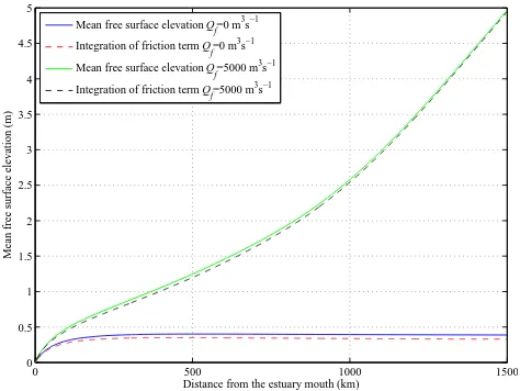
Figure 3 presents a comparison between the numerically calculated, tidally averaged water level and the values ob-tained from Eq. (26), both with (5000 m3s−1) and without river discharge. For simplicity, we calculated the tidally av-eraged friction using the Eulerian velocityUrather than the Lagrangean velocityV with (5000 m3s−1) and without river discharge. It can be seen from Fig. 3 that the correspondence between them is reasonable. The deviation is mainly due to the fact that we calculated the tidally averaged friction us-ing the Eulerian velocityU, instead of integrating the La-grangean velocityV as in Eq. (26). We can see from Fig. 3 that due to river discharge the residual water level slope is significantly increased, suggesting that the residual effects on the averaged water level is particularly important when river discharge is substantial.
6 Results
6.1 Analytical solutions of the new models
The different damping equations introduced above should be combined with the phase lag, scaling and celerity equa-tions of Table 2, to form the system of the hydrodynamic equations:
tan(ε)= λ
γ −δ, (28)
µ= sin(ε)
λ =
cos(ε)
γ −δ, (29)
λ2=1−δ (γ −δ). (30)
In this way we have a new set of four implicit analytical equa-tions that account for the effect of river discharge. As shown in Savenije et al. (2008), Eqs. (28) and (29) can be combined to eliminate the variableεto give
(γ −δ)2= 1
µ2 −λ
2. (31)
0 500 1000 1500
0 0.5 1 1.5 2 2.5 3 3.5 4 4.5 5
Distance from the estuary mouth (km)
Mean free surface elevation (m)
Mean free surface elevation Qf=0 m3s−1
Integration of friction term Qf=0 m3s−1
Mean free surface elevation Qf=5000 m3s−1
[image:7.595.309.546.62.240.2]Integration of friction term Qf=5000 m3s−1
Fig. 3. Tidally averaged free surface elevation calculated from the numerical model (solid lines) and evaluated through Eq. (26) both with and without river discharge for given values of K= 60 m1/3s−1, b= 352 km, ζ0= 0.2, h= 10 m, B0= 5000 m, Bmin= 300 m.
A fully explicit solution for the main dimensionless param-eters (i.e.µ,δ,λ,ε) can be derived in some cases (Toffolon et al., 2006; Savenije et al., 2008), but an iterative procedure is needed to obtain the solution in general. The following procedure usually converges in a few steps: (1) initially we assumeQf= 0 and calculate the initial values for the veloc-ity numberµ, celerity numberλand the tidal velocity am-plitudeυ (and hence dimensionless river discharge termϕ) using the analytical solution proposed in Cai et al. (2012a) (see Sect. 3); (2) taking into account the effect of river dis-chargeQf, the revised damping numberδ, celerity number
λ, velocity number µand velocity amplitudeυ (and hence
ϕ) are calculated by solving Eqs. (11), (30) and (31) using a simple Newton–Raphson method; (3) this process is repeated until the result is stable and then the other parameters (e.g.ε,
η,υ) are computed.
It is important to realize that the solutions for the depen-dent dimensionless parametersµ,δ,λandεare local solu-tions because they are obtained by the four implicit equa-tions that depend on local quantities that vary along the es-tuary (i.e. the local tidal amplitude to depth ratioζ, the local estuary shape number γ and the local friction number χ). To reproduce wave propagation correctly along the estuary, a multi-reach approach has to be used to follow along-channel variation, dividing the estuary in a number of reaches (e.g. Toffolon and Savenije, 2011). With the damping numberδ, it is possible to calculate a tidal amplitudeη1 at a distance
1x(e.g. 1 km) upstream by simple explicit integration of the damping number:
η1=η0+ dη
dx1x =η0+ η0ω δ
c0
0 0.2 0.4 0.6 0.8 1 −0.4
−0.2 0 0.2 0.4
Damping number
δ
0 0.2 0.4 0.6 0.8 1 0.45
0.5 0.55 0.6 0.65 0.7
Velocity number
μ
0 0.2 0.4 0.6 0.8 1 0.8
0.9 1 1.1 1.2 1.3
ϕ=Ur/υ
Celerity number
λ
0 0.2 0.4 0.6 0.8 1 33
33.5 34 34.5 35
ϕ=Ur/υ
Phase lag
ε
(
°
)
Hybrid Savenije Lorentz a)
c)
b)
[image:8.595.129.468.60.314.2]d)
Fig. 4. The main dimensionless parameters (damping numberδ, velocity numberµ, celerity numberλand phase lagε) obtained with the different analytical methods as a function of dimensionless river dischargeϕwithζ0= 0.1,γ= 1.5,χ= 20 andrS= 1.
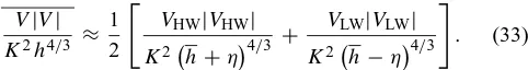
In a Lagrangean reference frame, tidally averaged friction can be estimated by the average of friction at HW and LW, based on the assumption that the water particle moves ac-cording to a simple harmonic, yielding
V|V|
K2h4/3 ≈ 1 2
"
VHW|VHW|
K2 h+η4/3
+ VLW|VLW|
K2 h−η4/3 #
. (33)
Substitution of different approximations of the friction term, described in the Sect. 4, into Eq. (33) and combination with Eq. (26) ends up with an equal number of analytical solutions for the tidally averaged depth along the estuary:
hnew(x)=h(x)+z(x), (34)
which modifies the estuary shape number. Making use of Eq. (34) an iterative procedure can be applied to obtain the tidal dynamics along the estuary accounting for the effect of the residual water level slope.
6.2 Comparison among different approaches
Table 3 summarizes the damping equations with and without the effect of river discharge for the different friction formu-lations, leading to different forms of the damping equation. The substitution ofϕ= 0 yields the same damping equations as in Table 2 (general case), as it can be derived by exploiting the phase lag and scaling equations (Cai et al., 2012a).
As an illustration, the relation between the dependent dimensionless parameters and the dimensionless river dis-charge ϕ is shown in Fig. 4 for given values of ζ0= 0.1,
γ= 1.5, χ= 2 and rS= 1. We can see that for increasing river discharge all the analytical models approach the same asymptotic solution, which is due to the fact that the ap-proximations to the quadratic velocityU|U|is close to U2
when the effect of tide is less important and the current no longer reverses. Actually, we can see that the parameter0
in the friction term in T1, T2 and T5 (see Table 3) tends to (4/3)ζ ϕ2/(µ λ) when ϕ approaching infinity. Moreover, it can be seen from Fig. 4 that the performance of the hy-brid model is close to the average of Lorentz’s and the quasi-nonlinear method, which is to be expected since the hybrid tidal damping represents a weighted average of these two so-lutions. In addition, we note that the different methods tend to converge for large values ofϕ.
It is important to realize that the different approaches use different expressions for the dimensionless friction f
(i.e. Eq. 9) as a result of the variation of the depth over time. While the effect of a variable depth is taken into account in the envelope method, the original Lorentz method assumes a constant depth in the friction term, which is the same as consideringζ= 0 in Eq. (9):
f0=g/
K2h1/3. (35)
[image:8.595.46.287.421.453.2]0 1 2 3 4 5 −3
−2 −1 0 1 2
Damping number
δ
0 1 2 3 4 5
0 0.2 0.4 0.6 0.8 1
Velocity number
μ
0 1 2 3 4 5
0.5 1 1.5 2 2.5 3
Friction number χ
Celerity number
λ
0 1 2 3 4 5
30 40 50 60 70
Friction number χ
Phase lag
ε
(
°
)
ϕ=0
ϕ=0.5
ϕ=1
ϕ=2
ϕ=5
a)
c)
b)
[image:9.595.128.468.61.316.2]d)
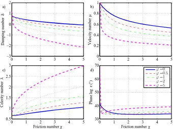
Fig. 5. Relationship between the main dimensionless parameters and the friction numberχ obtained by solving Eqs. (11) (with0=0H), (30) and (31) for different values of the dimensionless river discharge termϕwithζ0= 0.1,γ= 1.5 andrS= 1.
6.3 Sensitivity analysis
In this section we discuss the effect of changing the frictional and geometrical features of the estuary. Although in principle all the presented methods can be used, in the following we will consider the hybrid model, if not explicitly mentioned.
The relation between the dependent dimensionless param-eters (i.e. the damping numberδ, the velocity numberµ, the celerity numberλand the phase lagε) and the friction num-berχ for different values ofϕ is shown in Fig. 5 for given values ofζ0= 0.1,γ= 1.5 andrS= 1. In general, the river dis-charge intensifies the effect of friction, i.e. inducing more tidal damping (hence less velocity amplitude and wave celer-ity). The phase lagε= arcsin(µ λ)increases with increasing
ϕ except for smallχ when the values ofµ λare decreased. However, we can see that the curves show an anomaly for very small value ofχ. Ifχ is very small, the river discharge term in the numerator of the damping Eq. (11) is negligi-ble but becomes important inβ, defined in Eq. (12). For this case, an increase of the river discharge has an opposite ef-fect, particularly on the phase lag. In fact, for the case of a frictionless estuary (χ= 0) the damping Eq. (11) reduces toδ=µ2γ θ/(1+µ2β)in whichβ is decreased with river discharge.
The friction numberχis also a function ofζ (see Table 1). In order to illustrate the effect ofζ we introduce a modified (time-invariant) friction numberχ0as
χ0=χ
h
1−(4ζ /3)2i/ζ =rSg c0/
K2ω h4/3. (36)
Figure 6 describes the effect of the dimensionless tidal ampli-tudeζ for given values ofχ0= 20,γ= 1.5 andrS= 1. Larger
ζ intensifies the effect of river discharge and friction as well, which induces more tidal damping, less velocity amplitude and wave celerity, and increases the phase difference between HW and HWS (or LW and LWS). For small values ofζ, the phase lag decreases with increasing river discharge, also due to the effect onβ.
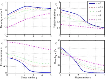
Figure 7 shows the effect of the estuary shape numberγ
on the main dimensionless parameters for different river dis-charge conditionsϕ and for given values of the other inde-pendent parameters (ζ0= 0.1,χ0= 20 andrS= 1). In general, the damping numberδ and the velocity numberµdecrease with river discharge, which means more tidal damping and less velocity amplitude. On the other hand, the celerity num-ber λ is increased (hence slower wave celerity) due to in-creasing river discharge. For the phase lagε, we can see from Fig. 7d that it decreases with river discharge for small val-ues ofγ while it increases for larger values ofγ. Cai et al. (2012a) found the same relationship between the main di-mensionless parameters and the friction number χ, which confirms our point that including river discharge acts in the same way as increasing the friction.
0 0.2 0.4 0.6 −15
−10 −5 0 5
Damping number
δ
0 0.2 0.4 0.6
0 0.2 0.4 0.6 0.8 1
Velocity number
μ
0 0.2 0.4 0.6
0 5 10 15
Dimensionless tidal amplitude ζ
Celerity number
λ
0 0.2 0.4 0.6
30 35 40 45
Dimensionless tidal amplitude ζ
Phase lag
ε
(
°
)
ϕ=0
ϕ=0.5
ϕ=1
ϕ=2
ϕ=5
a)
c)
b)
[image:10.595.128.468.61.316.2]d)
Fig. 6. Relationship between the main dimensionless parameters and the dimensionless tidal amplitudeζobtained by solving the Eqs. (11) (with0=0H), (30) and (31) for different values of the dimensionless river discharge termϕwithχ0= 20,γ= 1.5 andrS= 1, whereχ0is defined with Eq. (36).
0 1 2 3 4 5
−3 −2 −1 0 1
Damping number
δ
0 1 2 3 4 5
0 0.2 0.4 0.6 0.8 1
Velocity number
μ
0 1 2 3 4 5
0 0.5 1 1.5 2 2.5
Shape number γ
Celerity number
λ
0 1 2 3 4 5
0 20 40 60 80
Shape number γ
Phase lag
ε
(
°
)
ϕ=0
ϕ=0.5
ϕ=1
ϕ=2
ϕ=5
a)
c)
b)
d)
[image:10.595.128.467.400.656.2]0 200 400 600 800 1000 1200 1400 1600 1800 2000 0
0.5 1 1.5 2
Tidal amplitude (m)
ζ0=0.2
0 200 400 600 800 1000 1200 1400 1600 1800 2000 0
1 2 3 4 5
Distance from the estuary mouth (km)
Tidal amplitude (m)
ζ0=0.5 Num. Qf=5000 m 3s−1
Num. Qf=0 m3s−1
Ana. Q f=5000 m
3s−1 nodiv
Ana. Q
f=0 m
3s−1 nodiv
Ana. Q f=5000 m
3 s−1 div
Ana. Q
f=0 m
3s−1 div
Ana. U
r/υ, Qf=5000 m 3
s−1 div a)
[image:11.595.157.437.65.290.2]b)
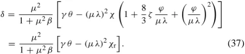
Fig. 8. Comparison between different analytical models and numerical results for given values ofK= 60 m1/3s−1,b= 352 km,h= 10 m, B0= 5000 m,Bmin= 300 m,ζ0= 0.2 (a) orζ0= 0.5 (b). The drawn black line represents the river velocity to tide velocity amplitude ratio. The label “nodiv” indicates the models without considering the residual water level slope, while “div” denotes the models accounting for it using the approach described in Sect. 5.
damping Eq. (11) can be written, with Eq. (14) for the case
ϕ < µ λ, as
δ= µ
2
1+µ2β
"
γ θ−(µ λ)2χ 1+ 8
3ζ ϕ µ λ +
ϕ µ λ
2!#
= µ
2
1+µ2β
h
γ θ −(µ λ)2χr
i
. (37)
This relationship shows that the effect of river discharge is basically that of increasing friction by a factor that is a function of ϕ. Expressing the artificial friction number as
χr=χ+1 χrprovides an estimation of the correction of the friction term
1 χr
χ =
8 3ζ
ϕ µ λ +
ϕ
µ λ 2
, (38)
which is needed to compensate for the lack of consider-ing river discharge. In fact, increasconsider-ing ϕ is analogous to changingχ, and the expected non-physical adjustment of the Manning–Strickler coefficientK can be estimated for mod-els that do not considerQf.
6.4 Comparison with numerical results
To investigate the performance of the analytical hybrid solu-tions, the results have been compared with a one-dimensional numerical model. Since we used Eq. (27) to describe the
width convergence along the estuary, the estuary shape num-ber accounting for width convergence becomes a function of distance:
γb =
c0 B0−Bminexp(−x/b)
b ωBmin+ B0−Bmin
exp(−x/b). (39)
When accounting for river discharge, it is necessary to in-clude depth divergence (i.e. the residual water level slope, which is particularly important if the bed is horizontal)
γd = −
c0
ω
1
h
dh
dx. (40)
Hence the combined estuary shape number reads
γ =γb+γd. (41)
[image:11.595.46.288.398.452.2]Table 4. Geometric and flow characteristics of the estuaries studied.
Tidal amplitude at the mouth (m) River dischargeQf(m3s−1) Estuary Reach Depthh Convergence Calibration Verification Calibration Verification
(km) (m) lengtha (km)
Modaomen
0–43 6.3 106
1.31 1.09 2259 2570
43–91 7 infinite 91–150 10.3 110
Yangtze
0–34 7 42
1.8 2.3 13 100 17 600
34–275 9 140 275–600 11 200
slightly better when including depth divergence due to resid-ual water level slope, especially in the upper reach of the es-tuary (this is due to the nonlinearity of the friction term). On the other hand, if river discharge is included, the analytical model requires taking account of depth divergence to accu-rately simulate the tidal damping. As the tidal amplitude to depth ratio ζ increases, the numerical simulations indicate that the deviation from the numerical results increases if we neglect the residual slope. Including depth divergence, the analytical model performs much better. However, the corre-spondence with numerical result is not perfect due to the fact that the analytical model does not account for wave distortion when the tide propagates upstream. More detailed comparion between analytical and fully nonlinear numerical results are presented in the Supplement.
6.5 Application to real estuaries
Using the damping Eq. (11) (in the hybrid version, hence
0=0H), the analytical model has been compared to observa-tions made in the Modaomen and Yangtze estuaries in China, where the influence of river discharge in the upstream part is considerable. The Modaomen estuary forms the downstream part of the West River entering the Pearl River Delta, with an annual river discharge of 7115 m3s−1at Makou (Cai et al., 2012b). The Yangtze estuary drains the Yangtze River basin with an annual mean river discharge of 28 310 m3s−1at Da-tong (Zhang et al., 2012).
The computation depends on the three independent vari-ables, i.e.γ,χ0andϕ. Given the flow boundary conditions (i.e. the tidal amplitude at the seaward boundary and river discharge at the landward boundary) and the geometry of the channel, the values ofγ,χ0andϕcan be computed. Hence, the set of four implicit analytical Eqs. (11) (with0=0H), (28), (29) and (30) can be solved by simple iteration. The tidal amplitude is obtained by numerical integration of the damping numberδover a length step (e.g. 1 km).
Table 4 presents the geometry and flow characteristics (considering two different cases for independent calibration and verification of the model) of the Modaomen and Yangtze on which the computations are based. The convergence
Table 5. Calibrated parameters of the estuaries studied.
Estuary Reach Storage Manning–Strickler Manning–Strickler (km) width friction friction
ratio K(m1/3s−1), K(m1/3s−1),
rS(−) Qf>0 Qf= 0
Modaomen
0–43 1.5 48 45
43–91 1.4 78 75
91–150 1.3 35 30
Yangtze
0–34 1.8 70 70
34–275 1 70 70
275–600 1 45 26
length of the cross-sectional area, which is the length scale of the exponential function, is obtained by fitting Eq. (1), where the parallel branches separated by islands are combined, as recommended by Nguyen and Savenije (2006) and Zhang et al. (2012). The calibrated parameters, including the stor-age width ratiorSand the Manning–Strickler frictionK, are presented in Table 5. In general, the storage width ratiorS ranges between 1 and 2 (Savenije, 2005, 2012). It is noted that a relatively small roughness value of K= 70 m1/3s−1 (Table 5) was used in the Yangtze estuary, which is due to the fact that it is a silt-mud estuary, while the bed consists of sands in the Modaomen estuary. The reason for the small roughness value ofK= 78 m1/3s−1used in the middle reach of the Modaomen estuary (43–91 km) is probably due to the effect of parallel branches (see Cai et al., 2012b).
[image:12.595.309.547.255.358.2]0 20 40 60 80 100 120 140 0
0.5 1 1.5
Tidal amplitude (m)
8−9 Feb. 2001
0 20 40 60 80 100 120 140 0
200 400 600
Travel time (min)
0 20 40 60 80 100 120 140 −1.5
−1 −0.5 0 0.5
Distance from the mouth (km)
Damping number
0 20 40 60 80 100 120 140 0
0.5 1 1.5
5−6 Dec. 2002 Qf=0 Q
f>0
obs.
0 20 40 60 80 100 120 140 0
200 400 600 HW Q
f=0
LW Q
f=0
HW Q
f>0
LW Q
f>0
HW obs. LW obs.
0 20 40 60 80 100 120 140 −1.5
−1 −0.5 0 0.5
Distance from the mouth (km) δ (Q
f=0)
δ (Q f>0)
a)
b)
c)
d)
e)
[image:13.595.130.469.64.322.2]f)
Fig. 9. Comparison of analytically calculated tidal amplitude (a, d), travel time (b, e) with measurements and comparison of two analytical models to compute the dimensionless damping number (c, f) on 8–9 February 2001 (calibration) and 5–6 December 2002 (validation) in the Modaomen estuary. The dashed line represents the model where river discharge is neglected. The continuous line represents the model accounting for the effect of river discharge. Both models used the same friction coefficients calibrated while considering river discharge.
of K= 30 m1/3s−1 to fit the data in the upstream part of Modaomen estuary (91–150 km). In Fig. 9, the new model accounting for the effect of river discharge is compared to the original model with the same roughness, but without river discharge. In the lower part of the estuary the models be-have the same (e.g. see the dimensionless damping number in Fig. 9c and f), but behave differently in the upper reach where the river discharge is dominant. Without considering river discharge, the model underestimates tidal damping upstream. In Fig. 10, we can see that the analytically calculated tidal amplitude in the Yangtze estuary is in good correspondence with the observed data on 21–22 December 2006 (calibra-tion) and 18–19 February 2003 (verifica(calibra-tion). For the travel time, the correspondence with observations at HW is very good, but the correspondence for LW shows a big devia-tion from the measurements, with an underestimadevia-tion of the celerity for LW. The reason for the deviation should prob-ably be attributed to significant tidal wave distortion due to the strong river discharge, which is critical for the assumption that the celerities at HW and LW times are symmetrical com-pared with the tidal average wave celerity (see Eq. A8 in Ap-pendix A). Without considering the river discharge, a much higher and unrealistic roughness (implying a lower value of
K= 26 m1/3s−1) would be necessary in the upstream part of the estuary (275–600 km) to compensate the influence of river discharge.
7 Conclusions
In this paper, we have extended the analytical framework for tidal hydrodynamics proposed by Cai et al. (2012a) by taking account of river discharge. With the envelope method (Savenije, 1998), different friction formulations considering river discharge can be used to derive expressions for the en-velopes at HW and LW and subsequently to arrive at the corresponding damping equations. When combined with the phase lag equation, the scaling equation and the celerity equation, these damping equations can be iteratively solved for the dimensionless parametersµ,δ,λandε, which are re-lated to tidal velocity amplitude, tidal damping, wave celer-ity, and phase lag, respectively. Thus, for given topography, friction, tidal amplitude at the seaward boundary and river discharge at the landward boundary, we can reproduce the main tidal dynamics along the estuary.
0 100 200 300 400 500 600 0
0.5 1 1.5 2
Tidal amplitude (m)
21−22 Dec. 2006
0 100 200 300 400 500 600 0
500 1000 1500
Travel time (min)
0 100 200 300 400 500 600 −1.5
−1 −0.5 0
Distance from the mouth (km)
Damping number
δ (Q f=0)
δ (Q f>0)
0 100 200 300 400 500 600 0
1 2 3
18−19 Feb. 2003 Qf=0 Q
f>0
obs.
0 100 200 300 400 500 600 0
500 1000 1500 HW Q
f=0
LW Q
f=0
HW Q
f>0
LW Q
f>0
HW obs. LW obs.
0 100 200 300 400 500 600 −1.5
−1 −0.5 0
Distance from the mouth (km) a)
b)
c)
d)
e)
[image:14.595.129.468.64.317.2]f)
Fig. 10. Comparison of analytically calculated tidal amplitude (a, d), travel time (b, e) with measurements and comparison of two analytical models to compute the dimensionless damping number (c, f) on 21–22 December 2006 (calibration) and 18–19 February 2003 (validation) in the Yangtze estuary. The dashed line represents the model where river discharge is neglected. The continuous line represents the model accounting for the effect of river discharge. Both models used the same friction coefficients calibrated while considering river discharge.
varying depth and only focus on the quadratic velocity. By using the envelope method, we are able to take this second nonlinear source into account and end up with a more com-plete damping equation accounting for river discharge.
We also note that the averaged water level tends to rise landward and that this effect has a considerable influence on tidal wave propagation, particularly when accounting for the effect of river discharge, since river discharge affects depth convergence and friction at the same time. An iterative ana-lytical method has been proposed to include the residual wa-ter level slope into the analysis, which significantly improved the performance of the analytical model.
With respect to e.g. Cai et al. (2012a), where we did not consider the effect of river discharge, this method is an im-provement that is important especially in the upstream part of the estuary where the influence of river discharge is con-siderable. This is clearly demonstrated by the application of the analytical model to two real estuaries (Modaomen and Yangtze in China), which shows that the proposed model fits the observations with realistic roughness value in the up-stream part, while the model without considering river dis-charge can only be fitted with unrealistically high roughness values.
Appendix A
Derivation of Lorentz’s damping equation incorporating river discharge using the envelope method
Using a Lagrangean approach as in Savenije (2005, 2012), the continuity equation can be written as
dV
dt =rs c h
dh
dt − c V
b +c V
1
η
dη
dx. (A1)
The momentum equation can also be written in a Lagrangean form, yielding
dV
dt +g ∂h
∂x +g (Ib−Ir)+g V|V|
K2h4/3 =0, (A2) whereIbis the bottom slope andIris the water level resid-ual slope resulting from the density gradient. Combination of these equations, and usingV= dx/dt, yields
rs
c V g h
dh dx −
c V g
1
b−
1 η
dη dx
+∂h
∂x +Ib−Ir+
V|V|
K2h4/3 =0.(A3)
Next, we condition Eq. (A3) for the situation of high water (HW) and low water (LW). The following relations apply to
dhHW dx −
dhLW dx =2
dη
dx, (A4)
dhHW,LW
dx =
∂h ∂x HW,LW , (A5)
dhHW dx +
dhLW dx ≈2
dh
dx, (A6)
withhHW≈h+η andhLW≈h−η. These three equations are acceptable ifη/h1.
The tidal velocities at HW and LW the following expres-sions can be expressed as
VHW ≈υsin(ε)−Ur, VLW ≈ −υsin(ε)−Ur, (A7) where the river flow velocityUris negative (it is in ebb direc-tion). Further we assume that wave celerity is proportional to the square root of the depth:
cHW √
hHW
≈ √cLW
hLW ≈ c
p h
. (A8)
In this example we use Lorentz’s linearization Eq. (21) of the bed friction (Lorentz, 1926), but also take into account the effect of the periodic variation of the hydraulic radius in the denominator of the friction term (i.e.K2h4/3). Combina-tion of Eqs. (A3), (A5), and the first of Eq. (A7) yields the following envelope for HW:
rscHW[υsin(ε)−Ur]
g h+η
dhHW dx −
cHW[υsin(ε)−Ur]
g 1 b − 1 η dη dx
+ dhHW dx +
1
K2 h+κ η4/3 1
4L0υ 2+ 1
2L1υ 2sin(ε)
= −Ib+Ir, (A9) whereκ= 1 corresponds to the time-dependent case, while
κ= 0 to the time-independent case. Similarly, for LW, com-bination of Eqs. (A3), (A5), and the second of Eq. (A7) yields the LW envelope:
−rscLW[υsin(ε)+Ur]
g h−η
dhLW dx +
cLW[υsin(ε)+Ur]
g 1 b − 1 η dη dx
+ dhLW dx +
1
K2 h−κ η4/3 1
4L0υ 2− 1
2L1υ
2sin(ε)= −I
b+Ir. (A10) Subtraction of these envelopes, using a Taylor series expan-sion ofh4/3, and taking into account the assumption on the wave celerity yields the following expressions:
rSc υsin(ε)
h
1
√
1+ζ dhHW
dx + 1
√
1−ζ dhLW
dx
−rSc Ur
h
1
√
1+ζ dhHW
dx − 1
√
1−ζ dhLW
dx
−
h
2c υsin(ε)+2c Ur
1−p1+ζ
i1
b− 1 η dη dx
+2gdη
dx +f
0
L1υ2sin(ε)
h
−κ2L0υ
2ζ
3h
=0, (A11) with the dimensionless friction factorf0defined as
f0 =g/K2h1/3 h1−(κ4ζ /3)2i −1
. (A12)
The parts between brackets in the first and second terms of Eq. (A11) can be replaced by the residual water level slope dh/dx defined in Eq. (A6) and dh/dx defined in Eq. (A4), respectively, providedζ1. Elaboration yields
1
η
dη
dx
θ−rs
ϕ
sin(ε)ζ + g η c υsin(ε)
= θ
b −rs
1
h
dh
dx
−L1 2 f
0 υ
h c+κL0 3 f
0υ ζ
h c
1
sin(ε). (A13)
The dimensionless parametersϕandθhave been defined in the main text. The first two terms on the right-hand side of Eq. (A13) represent the width and depth convergences and can be written as
θ b −rS
1
h
dh
dx = θ b +
rS
d ≈, θ
a. (A14)
Here, it has been assumed that both θ and rS are close to unity. Substitution of Eq. (A14) into Eq. (A13) yields
1
η
dη
dx
θ−rs
ϕ
sin(ε)ζ + g η c υsin(ε)
= θ
a − L1
2
f0 υ h c
+κL0
3 f
0υ ζ
h c
1
sin(ε). (A15)
Making use of the dimensionless parameters and adopting the scaling equation sin(ε)=µ λ, Eq. (A15) reduces to the following expression:
δ = µ
2 1+µ2
θ−rsϕ ζ /(µ λ)
γ θ −χ
1
2L1µ λ−κ 1 3L0ζ
, (A16)
or
δ= µ
2
1+µ2β (γ θ−χ µ λ 0L) , 0L=
L1 2 −κ ζ
L0
Appendix B
Derivation of the mean free surface elevation due to nonlinear frictional effect
Integration of the Lagrangean momentum equation (Eq. A2) over a tidal period leads to
V (t+T )−V (t )+g ∂ ∂x
t+T
Z
t
zdσ+gtt+T V|V|
K2h4/3dσ =0, (B1)
which can be simplified as
∂z ∂x = −
V|V|
K2h4/3, (B2)
when tidally averaged conditions achieve a regime configu-ration. Making use of the boundary conditionz= 0 atx= 0, integration of Eq. (B2) yields an expression for the mean free surface elevation:
z(x)= −
x
Z
0
V|V|
[image:16.595.125.526.91.689.2]K2h4/3dx. (B3)
Table A1. Nomenclature.
The following symbols are used in this paper
a convergence length of cross-sectional area;
A tidally averaged cross-sectional area of flow;
A0 tidally averaged cross-sectional area at the estuary mouth;
b convergence length of width;
B tidally averaged stream width;
B0 tidally averaged width at the estuary mouth; Bs storage width;
c wave celerity;
c0 celerity of a frictionless wave in a prismatic channel;
cHW wave celerity at HW; cLW wave celerity at LW; d convergence length of depth;
f friction factor accounting for the difference in friction at HW and LW;
f0 friction factor without considering the difference in friction at HW and LW;
F quadratic friction term;
FD Dronkers’ friction term accounting for river discharge;
FG Godin’s friction term accounting for river discharge;
Table A1. Continued.
The following symbols are used in this paper
FH hybrid friction term accounting for river discharge;
FL Lorentz’s friction term accounting for river discharge;
g acceleration due to gravity;
G0,G1,G2,G3 Godin’s coefficients accounting for river discharge;
h cross-sectional average depth;
h tidal average depth;
h0 tidally averaged depth at the estuary mouth;
hHW depth at HW; hLW depth at LW; Ib bottom slope;
Ir water level residual slope due to the density gradient;
K Manning–Strickler friction factor;
L0,L1 Lorentz’s coefficients accounting for river discharge;
p0,p1,p2,p3 Chebyschev coefficients accounting for river discharge;
Qf river discharge; rs storage width ratio;
t time;
T tidal period;
U cross-sectional average flow velocity; Ut tidal velocity;
Ur river velocity;
U0 the maximum possible velocity in Godin’s approach;
VHW velocity at HW; VLW velocity at LW;
V Lagrangean velocity for a moving particle;
x distance from the estuary mouth;
z free surface elevation;
α,β functions of dimensionless river discharge termϕ;
γ estuary shape number;
γb estuary shape number accounting for width convergence;
γd estuary shape number accounting for depth convergence;
0 damping parameter of quasi-nonlinear model;
Table A1. Continued.
The following symbols are used in this paper
0D damping parameter of Dronkers’ model; 0G damping parameter of Godin’s model; 0H damping parameter of hybrid model; δ damping number;
ε phase lag between HW and HWS (or LW and LWS); ζ tidal amplitude to depth ratio;
η tidal amplitude;
η0 tidal amplitude at the estuary mouth;
θ dimensionless term accounting for wave celerity not being equal at HW and LW;
κ coefficient that include the effect of time-dependent depth in the friction term;
λ celerity number; µ velocity number;
ρ water density;
υ tidal velocity amplitude;
φz,φU phase of water level and velocity;
ϕ dimensionless river discharge term accounting for river discharge;
χ friction number;
χ0 time-invariant friction number; ω tidal frequency.
Supplementary material related to this article is
available online at http://www.hydrol-earth-syst-sci.net/ 18/287/2014/hess-18-287-2014-supplement.pdf.
Acknowledgements. The authors would like to thank the two
anonymous referees for their valuable comments and suggestions, which have greatly improved this paper. The first author is finan-cially supported for his Ph.D. research by the China Scholarship Council with the project reference number of 2010638037.
Edited by: A. D. Reeves
References
Cai, H., Savenije, H. H. G., and Toffolon, M.: A new analytical framework for assessing the effect of sea-level rise and dredging on tidal damping in estuaries, J. Geophys. Res., 117, C09023, doi:10.1029/2012JC008000, 2012a.
Cai, H., Savenije, H. H. G., Yang, Q., Ou, S., and Lei, Y.: Influ-ence of river discharge and dredging on tidal wave propaga-tion; Modaomen estuary case, J. Hydraul. Eng., 138, 885–896, doi:10.1061/(ASCE)HY.1943-7900.0000594, 2012b.
Dronkers, J. J.: Tidal computations in River and Coastal Waters, Elsevier, New York, 1964.
Friedrichs, C. T. and Aubrey, D. G.: Tidal Propagation in Strongly Convergent Channels, J. Geophys. Res., 99, 3321–3336, 1994. Godin, G.: Modification of River Tides by the Discharge, J. Waterw.
Port C-ASCE, 111, 257–274, 1985.
Godin, G.: Compact Approximations to the Bottom Friction Term, for the Study of Tides Propagating in Channels, Cont. Shelf Res., 11, 579–589, 1991.
Godin, G.: The propagation of tides up rivers with special consid-erations on the upper Saint Lawrence river, Estuar. Coast. Shelf. S., 48, 307–324, 1999.
Horrevoets, A. C., Savenije, H. H. G., Schuurman, J. N., and Graas, S.: The influence of river discharge on tidal damping in alluvial estuaries, J. Hydrol., 294, 213–228, 2004.
Hunt, J. N.: Tidal oscillations in estuaries, Geo. J. Roy. Ast. Soc., 8, 440–455, doi:10.1111/j.1365-246X.1964.tb03863.x, 1964. Ippen, A. T.: Tidal dynamics in estuaries, part I: Estuaries of
rectan-gular section, in: Estuary and Coastline Hydrodynamics, edited by: Ippen, A. T., McGraw-Hill, New York, 1966.
Jay, D. A.: Green Law Revisited – Tidal Long-Wave Propagation in Channels with Strong Topography, J. Geophys. Res., 96, 20585– 20598, 1991.
Jay, D. A., Leffler, K., and Degens, S.: Long-Term Evolution of Columbia River Tides, J. Waterw. Port C-ASCE, 137, 182–191, 2011.
Kukulka, T. and Jay, D. A.: Impacts of Columbia River discharge on salmonid habitat: 1. A nonstationary fluvial tide model, J. Geo-phys. Res., 108, 3293, doi:10.1029/2002JC001382, 2003. Lanzoni, S. and Seminara, G.: On tide propagation in convergent
estuaries, J. Geophys. Res., 103, 30793–30812, 1998.
Leblond, P. H.: Tidal Propagation in Shallow Rivers, J. Geophys. Res., 83, 4717–4721, 1978.
Lorentz, H. A.: Verslag Staatscommissie Zuiderzee, Algemene Landsdrukkerij, The Hague, the Netherlands, 1926.
Nguyen, A. D. and Savenije, H. H. : Salt intrusion in multi-channel estuaries: a case study in the Mekong Delta, Vietnam, Hydrol. Earth Syst. Sci., 10, 743–754, doi:10.5194/hess-10-743-2006, 2006.
Parker, B. B.: The relative importance of the various nonlinear mechanisms in a wide range of tidal interactions, in: Tidal Hy-drodynamics, edited by: Parker, B. B., John Wiley, New York, 236–268, 1991.
Prandle, D.: Relationships between tidal dynamics and bathymetry in strongly convergent estuaries, J. Phys. Oceanogr., 33, 2738– 2750, 2003.
Savenije, H. H. G.: Lagrangian Solution of St Venants Equations for Alluvial Estuary, J. Hydraul. Eng., 118, 1153–1163, 1992. Savenije, H. H. G.: Determination of Estuary Parameters on Basis
of Lagrangian Analysis, J. Hydraul. Eng., 119, 628–642, 1993. Savenije, H. H. G.: Analytical expression for tidal damping in
allu-vial estuaries, J. Hydraul. Eng., 124, 615–618, 1998.
Savenije, H. H. G.: A simple analytical expression to describe tidal damping or amplification, J. Hydrol., 243, 205–215, 2001. Savenije, H. H. G.: Salinity and Tides in Alluvial Estuaries,
Else-vier, New York, 2005.
Savenije, H. H. G. and Veling, E. J. M.: Relation between tidal damping and wave celerity in estuaries, J. Geophys. Res., 110, C04007, doi:10.1029/2004JC002278, 2005.
Savenije, H. H. G., Toffolon, M., Haas, J., and Veling, E. J. M.: An-alytical description of tidal dynamics in convergent estuaries, J. Geophys. Res., 113, C10025, doi:10.1029/2007JC004408, 2008. Toffolon, M. and Savenije, H. H. G.: Revisiting linearized one-dimensional tidal propagation, J. Geophys. Res., 116, C07007, doi:10.1029/2010JC006616, 2011.
Toffolon, M., Vignoli, G., and Tubino, M.: Relevant parameters and finite amplitude effects in estuarine hydrodynamics, J. Geophys. Res., 111, C10014, doi:10.1029/2005JC003104, 2006.
Van Rijn, L. C.: Analytical and numerical analysis of tides and salinities in estuaries; part I: tidal wave propagation in convergent estuaries, Ocean Dynam., 61, 1719–1741, doi:10.1007/s10236-011-0453-0, 2011.
Vignoli, G., Toffolon, M., and Tubino, M.: Non-linear fric-tional residual effects on tide propagation, in: Proceedings of XXX IAHR Congress, vol. A, 24–29 August 2003, Thessaloniki, Greece, 291–298, 2003.
Zhang, E. F., Savenije, H. H. G., Wu, H., Kong, Y. Z., and Zhu, J. R.: Analytical solution for salt intrusion in the Yangtze Estuary, China, Estuar. Coast. Shelf. S., 91, 492–501, 2011.