Application of data based mechanistic modelling for flood forecasting at multiple locations in the Eden catchment in the National Flood Forecasting System (England and Wales)

www.hydrol-earth-syst-sci.net/17/177/2013/ doi:10.5194/hess-17-177-2013

© Author(s) 2013. CC Attribution 3.0 License.

Earth System

Sciences

Application of data-based mechanistic modelling for flood

forecasting at multiple locations in the Eden catchment in the

National Flood Forecasting System (England and Wales)

D. Leedal1, A. H. Weerts2,4, P. J. Smith1, and K. J. Beven1,3 1_{Lancaster Environment Centre, Lancaster University, Lancaster, UK} 2_{Deltares, P.O. Box 177, 2600 MH, Delft, The Netherlands}

3_{Geocentrum, Uppsala University, Uppsala, Sweden}

4_{Hydrology and Quantitative Water Management Group, Department of Environmental Sciences, Wageningen University,} Wageningen, The Netherlands

Correspondence to: D. Leedal ([email protected])

Received: 8 May 2012 – Published in Hydrol. Earth Syst. Sci. Discuss.: 8 June 2012 Revised: 29 October 2012 – Accepted: 15 December 2012 – Published: 18 January 2013

Abstract. The Delft Flood Early Warning System provides a versatile framework for real-time flood forecasting. The UK Environment Agency has adopted the Delft framework to de-liver its National Flood Forecasting System. The Delft sys-tem incorporates new flood forecasting models very easily using an “open shell” framework. This paper describes how we added the data-based mechanistic modelling approach to the model inventory and presents a case study for the Eden catchment (Cumbria, UK).

1 Introduction

Between 2004 and 2008 a component of the Flood Risk Man-agement Research Consortium (FRMRC) investigated data-based mechanistic (DBM) real-time flood forecasting and forecast uncertainty (Young et al., 2006). FRMRC phase 2 investigated uncertainty in inundation modelling using the Eden catchment as a test site. During this time, the UK Environment Agency launched the Risk-Based Probabilis-tic Fluvial Flood Forecasting study (Sene et al., 2009). The two projects exchanged ideas leading to the present au-thors developing a DBM module for the Delft Flood Early Warning System (Delft-FEWS). The module takes advantage of the Delft-FEWS open shell framework, which provides tried-and-tested code to drive models with real-time hydrol-ogy/meteorology data and permit data assimilation. The end

user is also given access to a sophisticated interface for visu-alizing and interacting with forecasts and data.

This paper provides a description of the DBM real-time flood forecasting method (Appendix A), a section describing the design and implementation of the FEWS module, and a case study building a semi-distributed DBM representation of the Eden catchment with forecast locations at Carlisle, which was extensively flooded in 2005 (Mayes et al., 2006; Neal et al., 2012), together with intermediate forecast points at Great Corby, Greenholme, Linstock, Cummersdale and Harraby Green.

2 Methods

2.1 The Eden catchment case study site

Allen et al. (2010) describes the geology and hydrogeology of the region as part of the Eden Demonstration Test Catch-ment Project.

The Upper Eden forms the largest sub-catchment at ∼

600 km2, with a number of tributaries originating from Mallerstang to the west and the Pennines to the east; both groups containing peaks over 700 m. The Lower Eden catch-ment contains a number of Pennine peaks on its eastern side, including Cross Fell (893 m). The western section is mainly improved farm land. The Eamont sub-catchment (158 km2) carries runoff from the central Lake District (in-cluding Helvellyn 950 m), where total rainfall is the high-est in the catchment (approximately 1700 mm yr−1). Two lakes regulate flow along the Eamont: Ullswater (884 ha) and Haweswater (387 ha). The Irthing sub-catchment (335 km2) is important from a flood management perspective as it is the only river carrying runoff from the northeast, close to the headwaters of the Tyne. This area was a major runoff generat-ing region durgenerat-ing the floodgenerat-ing in January 2005, contributgenerat-ing flows of 250 m3s−1. The Caldew sub-catchment (244 km2) is important for flooding at Carlisle as it drains from the high al-titude regions of Skiddaw (931 m), which is a region of steep impermeable igneous rock resulting in a fast catchment re-sponse. The Petteril sub-catchment (160 km2) is mainly im-proved lowland farms. The population within the catchment is approximately 240 000; the principal population centres are Carlisle, Penrith and Appleby.

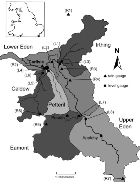
Forecast lead times in the catchment are limited to a max-imum of seven hours by steep relatively impermeable up-lands, areas of glacial moraines, high rainfall, and steep chan-nel geometry. Numerical weather predictions can extend this horizon but introduce further uncertainty. The distribution of rain-generating regions increases the forecasting challenge: Inputs from the central Lake District, Pennines, Skiddaw, and Kielder convolve to a complex signal observed at Carlisle. The UK Environment Agency closely monitors the catch-ment with a telemetered network of 31 level and 16 rainfall gauges generating a data field at 15 min intervals. Figure 1 shows the Eden catchment, sub-catchments and gauges used by the DBM model described in this paper.

2.2 The DBM flood forecasting model

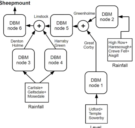
The FEWS DBM case study uses a network of 6 model nodes broadly representing the Eden sub-catchments. The configu-ration of the nodes is shown in Fig. 2 together with the En-vironment Agency gauge sites supplying input (rain or level) and output (level) to each node. Appendix A gives a descrip-tion of the DBM real-time flood forecasting method. The in-dividual transfer functions, input non-linearity functions and Kalman filter hyperparameters of the Eden DBM model were identified, estimated and optimised using theRIV, RIVID andSDPfunctions from the Captain™ toolbox (Taylor et al., 2007) and the Matlab™lsqnonlinfunction.

Appleby Carlisle

10 Kilometers

N

Penrith

rain gauge

level gauge (R1)

(R2)

(R3)

(R4)

(R5)

(R6)

(R7) (L1)

(L2)

(L3)

(L4)

(L5) (L6)

(L7)

(L8) Caldew

Petteril

Lower Eden Irthing

Upper Eden

Eamont

Fig. 1. The Eden catchment with locations of level () and rain

(N) gauges used by the DBM network model. Rain gauges R1 to

R7: Crewe Fell, Carlisle, Geltsdale, Harescough, Mosedale, High Row, and Udford; level gauges L1 to L8: Greenholme, Linstock, Great Corby, Sheepmount, Harraby Green, Cummersdale, Udford, and Temple Sowerby.

Fig. 2. Configuration of the nodes making up the Eden FEWS DBM module.

2.2.1 Forecast uncertainty

The Kalman filter algorithm described in Appendix A op-erates as an estimator for the probability distribution of the model states. Online data assimilation updates the state, er-ror covariance, and forecast estimates. Equation (A6) uses this information to estimate a variance for forecast error. The statistical assumptions of the Kalman filter and the form of the heteroskedastic variance model influence the accuracy of uncertainty estimates. Each is a simplification of the real sys-tem, and therefore calibration and ongoing testing should be used to monitor performance.

Uncertainty estimation is important in operational flood forecasting (see Beven, 2012, 289–311). Other research in-vestigating probabilistic forecasting within FEWS includes Weerts et al. (2011) describing the quantile regression method. The FEWS data visualisation screen presents uncer-tainty to the end user by displaying the 50th percentile fore-cast together with the 5 to 95th percentile range. Large uncer-tainty clearly communicates a volatile catchment or poorly performing model.

2.3 FEWS DBM module

2.3.1 Overview of FEWS

The FEWS open shell framework links a central database of hydrological and meteorological time series to an ever-growing inventory of forecasting models (Werner et al., 2013). An advanced set of utilities encapsulates data using extensible markup language (XML) and distributes these in a format specified by the model’s adapter module. The end

user is supplied with a graphical interface to view and inter-act with data.

The FEWS database adapter performs sophisticated merg-ing of time series to ensure that, where multiple pieces of information are available, observational data takes prece-dence followed by the most recently generated forecast val-ues (Deltares, 2010). This is important where upstream DBM nodes cascade forecasts to downstream nodes in order to achieve the maximum catchment lead time. In addition, FEWS substitutes the most logical value if a data point is missing or marked as corrupt. This improves operational ro-bustness.

The FEWS framework and DBM module are purely for operational use. We used the open source R language for the DBM module as it has all necessary functionality and the liberal terms of the GNU General Public Licence allow straightforward, cost-effective distribution (R Development Core Team, 2008). Model identification, estimation and opti-misation are carried out separately using the modeller’s tools of choice.

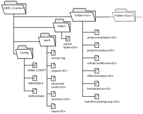
The FEWS DBM module specifies the directory tree and naming convention shown in Fig. 3. Each DBM node is fully described by the components in Ta-ble 1. This information is stored as name–value pairs in each node’s initialConditions file. The DBM model’s MAIN SCRIPT calls functions in turn that trans-fer the appropriate values from initialConditions to the mainProcessingLoop. This function per-forms Eqs. (A4), (A6), and (A9). At present, the mainProcessingLoopfunction is identical in each node and could have been a shared function; however, for maxi-mum flexibility, we chose to maintain a copy in each node so each can run a unique version of the Kalman filter algorithm in the future if required.

2.3.2 How the DBM module operates

The FEWS DBM nodes operate recursively: As sample pe-riod k becomes k−1, new observational data (uk, yk)are

assimilated to produce the output forecast horizon,yˆk+1 to ˆ

yk+δ, where δ is the maximum forecast lead time

avail-able at the node (see Appendix A). The algorithm also es-timates the uncertainty of each point in the forecast horizon,

Var(ykˆ+1|k, . . . ,ykˆ+δ|k). The nodes must be evaluated in the

order determined by the model cascade. Details of the algo-rithm are provided in Appendix A.

Table 1. The data structure describing a FEWS DBM node. Each node also includes a hard-coded input non-linearity function.

Data item Description

x Model states

ˆ

y Estimate for output

ˆ

σ2 Estimate of variance foryˆ

p, g, q_g Adaptive gain parameters as defined in Eq. (A9)

m Order of transfer function numerator

n Order of transfer function denominator

isLevel Boolean defining if input is level or rain

outOffset Offset value for the output

inOffset Vector of input offset(s)

δ Maximum forecast lead time

F,g,h,P,Q Kalman filter parameters as defined in Eq. (A4)

θ0,θ1 Heteroskedastic variance parameters as defined

in Eq. (A5)

adds little overhead and would allow time-varying parame-ters in the future.

At each time step FEWS extracts three data files from the central database: (1) observed input data made of present and

δpast values – for multiple input sites this file will have as many columns as required; (2) output data containing present andδ future time steps, with future values marked as miss-ing; and (3) auxiliary data (presently unused but available for future development). FEWS shifts the input data forward in time byδtime steps so the DBM module can always assume aδ of 0. The time shift appears complicated but is easily performed by FEWS, making the DBM processing straight forward.

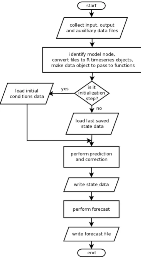
A forecast is generated for any segment of the output se-ries marked as missing; therefore, a forecast is always made for the finalδoutput values beyond the present sample time. The DBM module returns a file containing date, time, and a set of forecast percentiles (5, 50 and 95th by default). The FEWS adapter transfers this to the central database. Figure 4 shows the order of operation for a single time step. The pro-cess takes only seconds. The algorithm performs checks and logs progress at each stage of execution. The local machine can be powered down between samples if required.

3 Results for the Eden

3.1 Calibration

Calibration data ran from 9 September 2003 to 10 March 2005. The January 2005 flood event is sig-nificant in this period, with flows estimated to be in excess of 1500 m3s−1, the highest on record (see Mayes et al., 2006; Archer et al., 2007; Roberts et al., 2009). Using the DBM methodology, we identified and estimated the transfer function and input non-linearity for each of the 6 nodes pictured in Fig. 2. Each parameterisation had a reasonable

Fig. 3. The FEWS DBM module makes use of a directory and file naming convention. A catchment has a top levelDBM<name> di-rectory. Inside this, the functions of each node are contained within a separateFolder<ID> directory. TheConfigdirectory con-tains the main executable script and common processing functions. AWorkdirectory stores input, output and log files. Thestates

directory stores each node’s internal state data between execution steps. Individual scripts are labelled with “F” for a function, “D” for a data file, “T” for a text file, or “M” for the main executable script.

mechanistic interpretation: We consistently identified two dominant modes for rainfall to level models implying paral-lel fast and slow pathways (on the order of hours and days, respectively). Level to level nodes each returned a simple first-order response. The input non-linearity function for rainfall to level nodes roughly followed a logarithmic curve, indicating sensitivity to catchment antecedent conditions (increased runoff generation per unit of rainfall for a wet catchment).

We incorporated each node into the data assimilation al-gorithm shown in Appendix A and optimised the Kalman filter hyperparameters according to Smith et al. (2012a), cal-culating cost at the maximum forecast lead time. We man-ually specified adaptive gain hyperparameters to produce low-frequency, small amplitude forecast gain adjustments. Finally, we packaged the nodes into the full nested catch-ment structure. Example results for Sheepmount (Carlisle) are shown in Fig. 5.

3.2 Testing

Fig. 4. Flowchart showing the operations performed during a single data assimilation and forecast cycle. The initialization step loads the k=0 conditions.

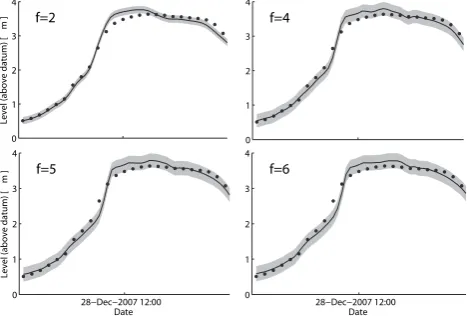
and 7 show detailed results for November 2009 at Sheep-mount and December 2007 at Linstock, respectively.

Figures comparing forecast and observation using a com-pressed time axis can appear overly convincing; instead we provide two alternative analyses of the Sheepmount data: (1) probability of detection (POD) and false alarm ratio (FAR) statistics (see Appendix B), and (2) Nash–Sutcliffe efficiency measures for the full data set and the sub-set above 3 m level. Using the Environment Agency flood warning thresholds for Sheepmount, we counted 57 threshold-crossing events. Table 2 gives a summary of POD and FAR results for a 6-h forecast at S6-heepmount. T6-he DBM module matc6-hed eac6-h threshold-crossing event. Data assimilation ensures the fore-cast tracks the observations reasonably well; occasionally the

0 2 4 6 8 10

Level (above datum) [

m

] _f=2

0 2 4 6 8 10

f=4

08−Jan−2005 09:00:00 0

2 4 6 8 10

Date

Level (above datum) [

m

] f=6

08−Jan−2005 09:00:00 0

2 4 6 8 10

Date f=7

Fig. 5. Results for the January 2005 event at Sheepmount (Carlisle). Dots show observed levels spaced at 2-h intervals; the solid line is thef-step ahead forecast (wheref=2, 4, 6 and 7 h); the grey area is the±2 standard deviation estimate of forecast uncertainty.

Table 2. 6-h lead-time performance measures for Sheepmount (Carlisle).

Statistic Mean Mean + s.d. Mean + 2 s.d.

POD 100 % 100 % 100 %

FAR 38.2 % 54 % 61 %

forecasts stray above a threshold not crossed by observations, increasing the false alarm rate. As expected, using the upper percentiles of the uncertainty range in the FAR calculation increases the false alarm ratio.

Table 3 gives Nash–Sutcliffe efficiency measures for the entire test data (35007 samples) and for the sub-set with a level over 3 m (334 samples). The global goodness-of-fit measure is excellent; however, it is considerably degraded for high-flow events. In theory, approximately 32 and 5 per-cent of observations should fall outside the 1 and 2 standard deviation ranges, respectively. The global data roughly con-forms to this expectation; again, the high-flow events demon-strate higher variance. While the heteroskedastic forecast un-certainty estimates go some way to addressing this, there are clearly further challenges. However, as Figs. 6 and 7 show, the DBM module provides valuable forecast information. It is worth noting the efficiency measure is reduced for high-flow events by a general tendency to over-predict level, which is arguably preferable from a precautionary perspective.

4 Conclusions

0 2 4 6 8

Level (above datum) [

m ] f=2 0 2 4 6 8 f=4

18−Nov−09 12:00 20−Nov−09 12:00 0 2 4 6 8 Date

Level (above datum) [

m

] f=6

18−Nov−09 12:00 20−Nov−09 12:00 0 2 4 6 8 Date f=7

Fig. 6. Results for the November 2009 event at Sheepmount (Carlisle). Dots show observed levels spaced at 2-h intervals; the solid line is thef-step ahead forecast (wheref =2, 4, 6 and 7 h); the grey area is the±2 standard deviation estimate of forecast un-certainty. 0 1 2 3 4

Level (above datum) [

m ] f=2 0 1 2 3 4 f=4 28−Dec−2007 12:00 0 1 2 3 4 Date

Level (above datum) [

m ] f=5 28−Dec−2007 12:00 0 1 2 3 4 Date f=6

Fig. 7. Results for the December 2007 event at Linstock (approx-imately 2 km upstream of Carlisle, maximum lead time 6 h). Dots show observed levels spaced at 2-h intervals; the solid line is the f-step ahead forecast (wheref =2, 4, 5 and 6 h); the grey area is the±2 standard deviation estimate of forecast uncertainty.

is based on the Kalman filter and is therefore probabilistic. The DBM module provides an estimate of forecast uncer-tainty. However, this study clearly illustrates the challenge of probabilistic flood forecasting by showing how the upper per-centiles of the uncertainty range generate a high false alarm rate while often underestimating the true variance of high-flow events.

We have also shown how the Delft-FEWS framework pro-vides a flexible and extensible mechanism for incorporating new flood forecasting models. Developing the DBM mod-ule for FEWS provided a test case for knowledge trans-fer between the research and operational environments. This process was quite straightforward, which demonstrates the strength of the FEWS philosophy.

Table 3. Summary of model performance for observations above 0 m (row 1) and 3 m (row 2). Column 3 (N–S) is the Nash–Sutcliffe efficiency measure. Columns 4 and 5 show the percentage of ob-servations outside the estimated 1 and 2 standard deviation range. Results are for the 6-h forecast at Sheepmount.

Observations Observations

Number of outside outside

Depth (m) observations N–S 1 s.d. 2 s.d.

0 35 007 0.98 17.3 % 5.1 %

3 334 0.45 74.2 % 34.3 %

Appendix A

DBM modelling and data assimilation

A1 DBM modelling

The fundamental component of a DBM model is the system transfer function; in discrete time

yk=B(z

−1₎

A(z−1₎uk−δ+ξk, (A1)

where B(z−1) and A(z−1) are polynomials of order m

andn, respectively:B(z−1)=b0+b1z−1+. . .+bmz−mand

A(z−1)=1+a1z−1+. . .+anz−n. Here z−1is the discrete

time backwards shift operator, i.e.z−iuk=uk−i;δis an

inte-ger value representing the time lag of the system, i.e. output (y) at timekis a response to the input stimulus (u) applied at timek−δ;ξkis a noise input representing all the stochastic components of the system not accounted for by the model. The model orders (mandn) and the polynomial coefficients are identified and estimated from time series data (see Young, 2011).

A2 Mechanistic interpretation

The steady-state gain and time constant of a first-order trans-fer function,b0/(1+a1z−1), are calculated respectively by

A3 Input non-linearity

The model input can be transformed to increase linearity be-tween input and output using

rk=F (uk,ykˆ +f), (A2)

whereris now the effective input formed as a function of the observed input (u) and the estimated level (yˆ) at forecast lead timef.

The DBM approach does not impose a specific form for the functionF. Beven et al. (2011) describe several candi-dates including power law, radial basis functions, piecewise cubic Hermite data interpolation, and Takagi–Sugeno fuzzy inference systems. The FEWS DBM module uses a function command so the modeller can develop the input non-linearity independently of the main body of the algorithm.

A4 State space representation

Equation (A3) represents Eq. (A1) in state space form.

x_k=Fx_k−1+grk−δ+ζk

yk=hTxk+ξk

, (A3)

wherexkis a vector of internal model states; the elements of

F,g, andhare determined by the transfer function parame-ters; andrk−δ is the suitably lagged effective input value.T

is the transpose operator. For operational flood forecasting,δ

is the identified advective time delay between input and out-put;ζk is a vector of process noise[ζ1,k· · ·ζn,k]T with each

element applied to the associatedninternal states;ξk is the

observation noise associated with the measurement. Here we make the simplifying assumption that the elements ofζkand ξk are zero mean, serially uncorrelated and statistically

in-dependent, normally distributed random variables with vari-ance at samplekspecified byζ1,k· · ·ζn,k andξk. Specifying

variance at each sample period allow a heteroskedastic mod-elling framework (see later). The state space representation is ideal for data assimilation using the Kalman filter (KF) (Kalman, 1960). Young (2002) describes a modified KF de-signed for the DBM model structure. Equation (A4) shows the two stage data assimilation process.

Forecast: ˆ

xk|k−1=Fxˆk−1+grk−δ

Pk|k−1=FPk−1FT+ ˆσk2Q

ˆ

yk|k−1=hTxˆk|k−1

Correction: ˆ

xk= ˆxk|k−1+Pk|k−1h[ ˆσ2+hTPk|k−1h]−1{yk− ˆyk|k−1}

Pk=Pk|k−1−Pk|k−1h[ ˆσ2+hTPk|k−1h]−1hTPk|k−1 ˆ

yk=hTxˆk (A4)

where Pk is the error covariance matrix associated with the

state estimate vectorxˆk; Q is a square matrix with diagonal

entries representing the ratio of variance of the process to observation noise for the model states (off-diagonal entries = 0), i.e. the diagonal elements of Q are[ζ1,k

ξk · · ·

ζn,k

ξk ];σˆ

2

k is an

estimate of the heteroskedastic observation noise variance at samplekcalculated using the empirical formula

ˆ

σ_k2=θ0+θ1yˆk2, (A5)

whereθ0andθ1are hyperparameters determining the degree of inflation in observation uncertainty for increasing ampli-tude of the observation. Iterating the forecast step of Eq. (A4) generates thef-step forecast (wheref≤δ). The variance of the forecastyˆk+f|kis estimated by

Var(yˆk+f|k)= ˆσk2+h

T_P

k+f|kh. (A6)

A5 Hyperparameter optimisation

The hyperparameters in Eqs. (A4) and (A5) are multiplica-tive and cannot be optimised directly. Smith et al. (2012a) show optimisation up to proportionality ifθ0is fixed at 1 and the optimisation is limited to a scaledθ1and the diagonal el-ements of Q. The result gives a ratio for distributing process noise between the state variables, and a scaledθ1. To imple-ment, replace Eq. (A5) with

ˆ

σ_k2=cscale(1+θ1yˆk2), (A7)

then, assuming normally distributed model residuals, esti-matecscaleusing

yk− ˆyk

ˆ

qk|k−f

∼N (0, cscale). (A8)

A6 Adaptive gain

Finally, we include an adaptive gain mechanism such that the true output(yk)is assumed to be a product of a time varying

scalar gain term(gk)and the model estimate(yˆk). The gain

operates independently of the main data assimilation scheme and is designed to account for long-term bias in the equilib-rium response of the catchment such as seasonal variations or gradual adjustments to channel geometry. The time variation in the gain term is modelled as a random walk process again employing a Kalman filter algorithm to update the gain state online in response to observed level data. The adaptive gain is fixed during thef-step forecast period as no new level data is available for assimilation. The modified scalar Kalman fil-ter proposed by Young (2002) is used for the adaptive gain:

pk|k−1=pk−1+qg

pk=pk|k−1−

p2_k|k−1yˆ2_k

1+pk|k−1yˆk2 ˆ

gk= ˆgk−1+pkyˆk{yk− ˆgk−1yˆk}

, (A9)

wherepk is the error variance term associated with the gain

how quickly the gain is allowed to adjust; ykˆ is the esti-mate of level prior to applying the adaptive gain; andyk is the observed level. In the Eden example described in this pa-per, theqgterms were tuned manually taking values between

1×10−2and 1×10−5, depending on the characteristics of the node. It is useful to note that the adaptive gain method can be used on its own as a form of data assimilation for any deterministic model (e.g. Smith et al., 2012b).

Appendix B

POD and FAR calculation

Probability of detection (POD) and false alarm ratio (FAR) (see Sene et al., 2009, p. 25) gauge a model’s forecast skill. When a threshold crossing is forecast, that prediction can turn out to be either (a) correct, or (b) wrong. Alternatively, a forecast of a threshold not crossed can turn out to be (c) wrong, or (d) correct. POD and FAR are calculated by summing each outcome over a number of events, and then POD =_a+a_c and FAR =_b+b_a.

Acknowledgements. This research was carried out as part of RPA9 and SWP1 of the Flood Risk Management Research Consortium (FRMRC) phase 1 and 2. The principal sponsors of FRMRC are the Engineering and Physical Sciences Research Council (EPSRC) in collaboration with the Environment Agency (EA), the Northern Ireland Rivers Agency (DARDNI), the United Kingdom Water Industry Research Organisation (UKWIR), the Scottish Government (via SNIFFER), the Welsh General Assembly (WAG) through the auspices of the Defra/EA, and the Office of Public Works (OPW) in the Republic of Ireland. The data was supplied by the Environment Agency. Deltares provided access to the FEWS National Flood Forecasting System (NFFS) and expert support and advice during the development of the DBM module. The work was also supported by the UK Environment Agency project SC080030 Risk-based probabilistic fluvial flood forecasting for integrated catchment models.

Edited by: Y. Liu

References

Alfieri, L., Smith, P. J., Thielen-del Pozo, J., and Beven, K. J.: A staggered approach to flash flood forecasting – case study in the C´evennes region, Adv. Geosci., 29, 13–20, doi:10.5194/adgeo-29-13-2011, 2011.

Allen, D., Newell, A., and Butcher, A.: Preliminary review of the geology and hydrogeology of the Eden DTC sub-catchments, available at: http://nora.nerc.ac.uk/12788/1/OR10063.pdf (last access: 10 November 2012), British Geological Survey Open Re-port, OR/10/063, 2010.

Archer, D., Leesch, F., and Harwood, K.: Learning from the extreme River Tyne flood in January 2005, Water Environ. J., 21, 133– 141, 2007.

Beven, K.: Rainfall-Runoff Modelling: The primer, Second Edition, John Wiley and Sons, Ltd, Chichester, UK, 2012.

Beven, K., Leedal, D., Smith, P., and Young, P.: Identification and Representation of State Dependent Non-linearities in Flood Fore-casting Using the DBM Methodology, in: System Identification, Environmental Modelling and Control Systems Design, edited by: Wang, L. and Garnier, H., 341–366, Springer Verlag, 2011.

Deltares: Data handling in Delft-FEWS, available at:

http://publicwiki.deltares.nl/display/FEWSDOC/02+Data+ Handling+in+DELFT-FEWS (last access: 10 November 2012), 2010.

Kalman, R.: A new approach to linear filtering and prediction prob-lems, J. Basic Eng.-T. ASME, 82, 35–45, 1960.

Leedal, D., Beven, K., Young, P., and Romanowicz, R.: Data as-similation and adaptive real-time forecasting of water levels in the river Eden catchment, UK, in: Flood Risk Management: Re-search and Practice, edited by: Samuels, P., p. 221, CRC Press, 2009.

Mayes, W., Walsh, C., Bathurst, J., Kilsby, C., Quinn, P., Wilkinson, M., Daugherty, A., and O’Connell, P.: Monitoring a flood event in a densely instrumented catchment, the Upper Eden, Cumbria, UK, Water Environ. J., 20, 217–226, 2006.

Neal, J., Keef, C., Bates, P., Beven, K., and Leedal, D.: Probabilistic flood risk mapping including spatial dependence, Hydrol. Pro-cess., online first: doi:10.1002/hyp.9572, 2012.

R Development Core Team: R: A Language and Environment for Statistical Computing, R Foundation for Statistical Computing, Vienna, Austria, available at: http://www.R-project.org, ISBN:3-900051-07-0, 2008.

Roberts, N., Cole, S., Forbes, R., Moore, R., and Boswell, D.: Use of high-resolution NWP rainfall and river flow forecasts for ad-vance warning of the Carlisle flood, north-west England, Meteo-rol. Appl., 16, 23–34, 2009.

Romanowicz, R., Young, P., and Beven, K.: Data assimilation and adaptive forecasting of water levels in the river Severn catchment, United Kingdom, Water Resour. Res., 42, W06407, doi:10.1029/2005WR004373, 2006.

Sene, K., Weerts, A., Beven, K., Moore, R., Whitlow, C., and Young, P.: Risk-based probabilistic fluvial flood forecasting for integrated catchment models-Phase 1 Report, 2009.

Smith, P., Beven, K., and Horsburgh, K.: Data-based mechanistic modelling of tidally affected river reaches for flood warning pur-poses: an example on the River Dee, UK, Q. J. Roy. Meteorol. Soc., online first, doi:10.1002/qj.1926, 2012a.

Smith, P. J., Beven, K. J., Weerts, A. H., and Leedal, D.: Adaptive correction of deterministic models to produce probabilistic fore-casts, Hydrol. Earth Syst. Sci., 16, 2783–2799, doi:10.5194/hess-16-2783-2012, 2012b.

Spencer, P., Boswell, D., Davison, I., and Lukey, B.: Flood fore-casting using real time hydraulic and other models: lessons from the Carlisle flood in January 2005, in: 41th DEFRA Flood and Coastal Management Conference, The University of York, 4–6, 2006.

Taylor, C., Pedregal, D., Young, P., and Tych, W.: Environmental time series analysis and forecasting with the Captain toolbox, Environ. Modell. Softw., 22, 797–814, 2007.

Sys-tem (England and Wales), Hydrol. Earth Syst. Sci., 15, 255–265, doi:10.5194/hess-15-255-2011, 2011.

Werner, M., Schellekens, J., Gijsbers, P., van Dijk, M., van den Akker, O., and Heynert, K.: The Delft-FEWS flow forecasting system, Environ. Modell. Softw., 40, 65–77, doi:10.1016/j.envsoft.2012.07.010, 2013.

Young, P.: Advances in real–time flood forecasting, Philos. T. R. Soc. Lond., 360, 1433–1450, 2002.

Young, P.: Recursive Estimation and Time-Series Analysis: An In-troduction for the Student and Practitioner, Springer, 2011. Young, P., Romanowicz, R., and Beven, K.: Updating algorithms in