On selection of the optimal data time interval for real time hydrological forecasting

(1)

www.hydrol-earth-syst-sci.net/17/3639/2013/ doi:10.5194/hess-17-3639-2013

Hydrology and

Earth System

Sciences

On selection of the optimal data time interval for real-time

hydrological forecasting

J. Liu1,2and D. Han2

1_{State Key Laboratory of Simulation and Regulation of Water Cycle in River Basin, China Institute of Water Resources and} Hydropower Research, Beijing 100038, China

2_{Water and Environmental Management Research Centre, Department of Civil Engineering, University of Bristol,} Bristol BS8 1TR, UK

Correspondence to: J. Liu (jia.liu@iwhr.com)

Received: 22 August 2012 – Published in Hydrol. Earth Syst. Sci. Discuss.: 26 September 2012 Revised: 25 June 2013 – Accepted: 14 August 2013 – Published: 30 September 2013

Abstract. With the advancement in modern telemetry and

communication technologies, hydrological data can be col-lected with an increasingly higher sampling rate. An impor-tant issue deserving attention from the hydrological com-munity is which suitable time interval of the model input data should be chosen in hydrological forecasting. Such a problem has long been recognised in the control engineer-ing community but is a largely ignored topic in operational applications of hydrological forecasting. In this study, the in-trinsic properties of rainfall–runoff data with different time intervals are first investigated from the perspectives of the sampling theorem and the information loss using the dis-crete wavelet transform tool. It is found that rainfall signals with very high sampling rates may not always improve the accuracy of rainfall–runoff modelling due to the catchment low-pass-filtering effect. To further investigate the impact of a data time interval in real-time forecasting, a real-time forecasting system is constructed by incorporating the prob-ability distributed model (PDM) with a real-time updating scheme, the autoregressive moving-average (ARMA) model. Case studies are then carried out on four UK catchments with different concentration times for real-time flow forecasting using data with different time intervals of 15, 30, 45, 60, 90 and 120 min. A positive relation is found between the forecast lead time and the optimal choice of the data time interval, which is also highly dependent on the catchment concentration time. Finally, based on the conclusions from the case studies, a hypothetical pattern is proposed in three-dimensional coordinates to describe the general impact of the data time interval and to provide implications of the selection

of the optimal time interval in real-time hydrological fore-casting. Although nowadays most operational hydrological systems still have low data sampling rates (daily or hourly), the future is that higher sampling rates will become more widespread, and there is an urgent need for hydrologists both in academia and in the field to realise the significance of the data time interval issue. It is important that more case studies in different catchments with various hydrological forecast-ing systems are explored in the future to further verify and improve the proposed hypothetical pattern.

1 Introduction

(2)

3640 J. Liu and D. Han: Optimal data time interval for real-time hydrological forecasting

(Freer et al., 1996; Krzysztofowicz, 1999, 2002; Tamea et al., 2005; Mantovan and Todini, 2006; Chen and Yu, 2007), as well as numerical weather prediction (NWP), which provides precipitation forecasts as the input of the forecasting system and allows for an extension of the forecast lead time (Cloke and Pappenberger, 2009; Wood and Schaake, 2008; Lin et al., 2002, 2006, 2010). However, no matter how advanced these methods are, and how much they can improve the forecasting results, they all depend on a reliable hydrological forecasting model, which normally consists of a rainfall–runoff model (either lumped, distributed or semi-distributed) together with a real-time updating scheme. When constructing the fore-casting system, there is an important issue that cannot be avoided, i.e. the selection of the time interval of the model input data (e.g. the rainfall, streamflow and evaporation, etc.) used to drive the system, which is, however, mostly ignored by the hydrological community in operational applications. A simple search using Google Scholar with the keywords “hydrological forecasting” reveals 84 500 articles covering scientific publications on hydrological forecasting in the last 30 yr and beyond. However, there is seldom the mention of “time interval”. Not only “data time interval” is seldom men-tioned; also “model time interval” and “model time step” are rarely mentioned.

Many real-time hydrological forecasting systems tend to use data as they are originally measured. Take the National Flood Forecasting System (NFFS) (Werner et al., 2009) of the Environmental Agency (EA) as an example. The NFFS system provides a platform capable of using of a standard set of EA-approved models to make real-time flood fore-casts for eight regions in England and Wales. It has roughly been pointed by Sene et al. (2009) that for large, slowly re-sponding rivers, an hourly time step is sufficient, while a shorter time step is required on flashier catchments. How-ever, since rainfall–runoff data are measured at a minimal time interval of 15 min in the UK, the 15 min time step is nor-mally adopted when forecasts are made by the NFFS system (Sene et al., 2010). Examples are taken from NFFS in the study of Weerts et al. (2011) to estimate the predictive un-certainty in flood forecasting. A variety of catchments with different sizes (30–1000 km2) and hydrological behaviours are selected from three EA regions: the North East, Mid-lands and Thames regions, which are respectively modelled by three rainfall–runoff models: the probability distributed model (PDM) (Moore, 2007), MCRM (Midlands Catchment Runoff Model) (Bailey and Dobson, 1981) and nested TCMs (Thames Catchment Models) models (Wilby et al., 1994). The observed rainfall–runoff data are directly used for cal-ibration and forecasting with different lead times (0–48 h). Similarly, in the study of Schellekens et al. (2011), the whole Thames region is chosen to test the use of MOGREPS en-semble rainfall forecasts in the NFFS system. A configura-tion of 148 TCM models is employed with a deterministic 15 min time step to make forecasts for the range of 0–3 days.

A distinction should be made here between the sampling interval of the hydrological measurements and the time in-terval of the model input data. A sampling inin-terval is deter-mined by the instruments (e.g. the rain gauge and the flow gauge) and could be as frequent as the instrument can af-ford, while the time interval of the model input data refers to the time interval of the hydrological data (e.g. rainfall and streamflow) used to construct the forecasting system, or equivalently, the time step at which the forecasting system is operating. For an easier quotation, we use the term “data time interval” hereafter to refer to the interval of the model input data, and use “sampling interval” to represent the raw hydrological measurements.

(3)

time interval in either linear or nonlinear systems may lead to a dramatic increase of the variances for the model param-eter estimates. It was also pointed out by Clark and Kavetski that for highly nonlinear systems, the optimal time interval should be even smaller than the system time constant (i.e. the catchment concentration time) due to the problem of solv-ing the nonlinear ordinary differential equations numerically (Clark and Kavetski, 2010; Kavetski and Clark, 2010).

In the past decade, this issue has begun to gain attention from hydrologists in academia. A general consensus has been reached that the parameters, simulation results and process representations of the hydrological models are inherently and strongly time-step-dependent (e.g. Duan et al., 2006; Merz et al., 2009, 2011). More than a decade ago, Schaake et al. (1996) developed a simple water balance model and tested its sensibility for operating at time steps different from what it was calibrated at. It was recommended that in order to ob-tain the best performance, the model should be calibrated at the same time step as the one used for operation. Fol-lowing this, a number of studies have been carried out on the time-step dependency of the hydrological model param-eters (Finnerty et al., 1997; Tang et al., 2007; Littlewood and Croke, 2008; Wang et al., 2009; Cho et al., 2009; Kavet-ski et al., 2011), for its implications in regionalisation at ungauged catchments or climate impact analysis, etc. How-ever, the impact of the model time step, or using the equiv-alent expression in this study, i.e. the time interval of the model input data, on the inference of the catchment struc-ture, model parameters and, more generally, the catchment behaviour remains poorly understood (Kavetski et al., 2011). Furthermore, in operational applications, scientists are more interested in the improvement of the model accuracy and the appropriate use of the observational data rather than reduc-ing the time dependency of the model parameters. Although the utilisation of hydrological observations at appropriately fine resolutions is advocated by Wagener et al. (2010), there still remains a lack of general guidance allowing for hydrolo-gists to better cope with this time interval issue in operational applications. Moreover, most of the previous studies are fo-cused on the use of hydrological models for simulation. With respect to hydrological forecasting, this issue becomes more complicated by the involvement of another temporal concept – the forecast lead time. In such cases, a suitable choice of the time interval of the model input data is much more important, and deserves further considerations.

In the area of hydrological forecasting, it has been firstly addressed in the work of Remesan et al. (2010) that when the artificial neural network (ANN) is used for real-time flood forecasting, there is an optimal time interval for the input data. It has been found that the 30 min interval can produce more accurate forecast results than the 15, 60 and 120 min intervals in the Brue catchment of the UK, and the signif-icance of the time interval impact on the forecasting accu-racy is more prominent for longer lead times than shorter ones. The results are quite meaningful to data-driven

mod-els, the performances of which are highly time-dependent, and improper data inputs could easily lead to overfitting (a serious weakness associated with such models). However, a question might arise: will this “optimal time interval” still exist for forecasting made by using the more widely applied conceptual rainfall–runoff models? The conceptual rainfall– runoff models encompass a broad spectrum of plausible de-scriptions of the physical rainfall–runoff processes, which are found to be both reliable and effective in various situa-tions, especially for real-time hydrological forecasting (Bell et al., 2001). The purpose of this study is to explore the gen-eral impact of the data time interval on hydrological forecast-ing usforecast-ing the conceptual rainfall–runoff model and a real-time updating scheme.

In this study, the intrinsic properties of observed rainfall– runoff data with different sampling intervals are firstly inves-tigated from the perspective of the information loss using the spectral analysis tool of discrete wavelet transform. Then the impact of a data time interval on the accuracy of real-time hydrological forecasting is examined through case studies. A real-time forecasting system is constructed by incorporating the PDM with a real-time updating scheme, the autoregres-sive moving-average (ARMA) model. Rainfall–runoff data with different time intervals of 15, 30, 45, 60, 90 and 120 min are taken from four UK catchments with different drainage areas, and then used to drive the constructed forecasting sys-tem. Forecasts are made using different time-interval data with the forecast lead time ranging from 1 to 12 h. The under-lying relation between the optimal data time interval and the forecast lead time is investigated, and the implications of the catchment concentration time on the selection of the optimal time interval is further discussed. Finally, based on the spec-tral analyses of the rainfall–runoff observations and the fore-casting results from the case studies, a hypothetical pattern is proposed to describe the general impact of the data time interval and to provide hints on the selection of the optimal time interval in real-time hydrological forecasting.

2 Material and methods

2.1 Spectral analysis for rainfall–runoff data with different time intervals

2.1.1 Sampling methods for rainfall–runoff

observations

(4)

37

Figures

(a) 15min data

0 10 20 30 40 R unof f ( m 3/s ) 0 4 8 12 R a in fa ll in te n s it y (m m /h r)

(b) 30min data

0 10 20 30 40 R u n o ff ( m 3/s ) 0 4 8 12 R a in fa ll in te n s it y (mm/ h r)

(c) 60min data

0 10 20 30 40 R unof f ( m 3/s ) 0 4 8 12 R a in fa ll in te n s it y (mm/ h r)

(d) 120min data

0 10 20 30 40 R unof f ( m 3/s ) 0 4 8 12 R a in fa ll i n te n s it y (m m /h r)

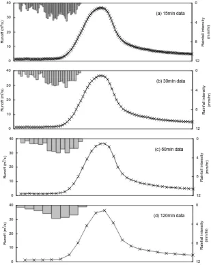
[image:4.595.143.452.63.451.2]

Figure 1 Observed rainfall-runoff data with different sampling intervals of (a) 15min, (b) 30min, (c) 60min and (d) 120min.

Fig. 1. Observed rainfall–runoff data with different sampling intervals of (a) 15 min, (b) 30 min, (c) 60 min and (d) 120 min.

a sampling data function where the value of the continuous functionQ(t )in thejth time intervalQj is given simply by

the instantaneous value ofQ(t )at timej 1t:

Qj =Q(tj)=Q(j 1t ). (1)

The other way is to adopt a pulse data function, in which the value of the discrete time functionQj is given by the area

under the continuous functionQ(t ):

Qj = j 1t

Z

(j−1)1t

Q(t )dt . (2)

The two principal variables of interest in hydrology, stream-flow and rainfall, are measured as sampled data series and pulse data series, respectively (Chow et al., 1988). When the values of streamflow and rainfall are recorded by gauges at a given instant, the flow gauge value represents the flow rate at that instant (in dimensions of (L3/T)), while the rainfall

gauge value is the accumulated depth of rainfall (in dimen-sion of (L) standing for the volume of rainfall (L3)) which has occurred up to that instant.

(5)

The theorem, often known as the sampling theorem, provides a lower boundary of the sampling frequency and thus an up-per boundary of the sampling interval as a sufficient condi-tion for a perfect reconstruccondi-tion of the original signal in the absence of observational noise:

fs>2B, (3)

or equivalently,

B < fs/2, (4)

wherefs is the sampling frequency and B is the one-sided baseband bandwidth of the band-limited original signal.fs/ 2 is defined as the Nyquist frequency, which is a property of the sampled system. If the condition is not satisfied, then the part of information of the original signal with frequencies be-yond the Nyquist interval (−fs/ 2,fs/ 2) will be lost during sampling, and the spectral density inside the interval can be distorted in the process of signal reconstruction, which will lead to the phenomenon of aliasing (Mitchell et al., 1988). On the other hand, if the frequency of the downsampled data is higher than twice the bandwidth of the original signal, then the information loss can be neglected, and the original signal can also be successfully reconstructed. This has, at least from the theoretical aspect of the signal reconstruction, refuted the intuition of many modellers, and demonstrated that choosing a relatively larger time interval will not always deteriorate the modelling results.

2.1.2 Discrete wavelet transform

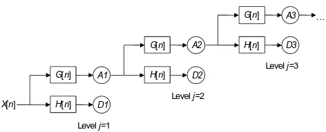
In order to further investigate the information content of the observed rainfall–runoff data with different sampling inter-vals before they are used in hydrological forecasting, discrete wavelet transform (DWT) is applied to investigate the energy distribution of the observed rainfall–runoff data in different frequency domains. DWT is a powerful mathematical tool for the spectral analysis of discrete signals, which is more ef-ficient than the Fourier transform in studying non-stationary time series (Meyer, 1993; Polikar, 1999). A most popular and efficient way to implement DWT is the Mallat decomposition algorithm (Mallat, 1989), the process of which is illustrated in Fig. 2.

The decomposition levelj is associated with a frequency band1F calculated based on the sampling frequencyfs:

2−j−1fs≤1F≤2−jfs. (5)

The original signal is first decomposed into an approxima-tion and an accompanying detail. The detail contains the high-frequency components of the signal within the fre-quency band 1F, while the approximation represents the low-frequency components below the band. Table 1 gives the corresponding frequency bands of the six wavelet de-composition levels for a 15 min data series obtained by using

38

X[n]

G[n]

H[n]

A1

D1

G[n]

H[n]

A2

D2

G[n]

H[n]

A3

D3

Level j=1

Level j=2

[image:5.595.310.546.60.156.2]

Level j=3 …

Figure 2 Process of the discrete wavelet decomposition following the Mallat decomposition

algorithm. X[n] is a discrete signal with n samples, passing though a low-pass filter G and a high-pass filter H with impulse responses of G[n] and H[n], respectively. A1, A2, A3 and D1, D2, D3 are the decomposed approximations and details on level j = 1, 2, 3….

Groundwater storage Surface storage

Rainfall (fc)

ET (be)

Direct runoff

Recharge

Qs

Qb

Surface runoff

Baseflow Probability-distributed

soil moisture storage

Q

(cmin, cmax, b) (kg, bg, St)

(k1, k2)

(kb)

(qc, τd)

Figure 3 Conceptual structure of the PDM model. The 13 model parameters to be calibrated

are in the brackets.

Fig. 2. Process of the discrete wavelet decomposition following the

Mallat decomposition algorithm.X[n] is a discrete signal withn

samples, passing though a low-pass filterGand a high-pass filterH

with impulse responses ofG[n] andH[n], respectively. A1, A2, A3

and D1, D2, D3 are the decomposed approximations and details on

levelj= 1, 2, 3. . .

Eq. (5). The decomposition process is iterated, with succes-sive approximations being decomposed in turn so that the original signal is broken down into many lower-resolution components. In this study, the decomposition is carried out by decomposing 1 yr observed rainfall–runoff data into six decomposition levels using the Daubechies wavelet of or-der 10, 12 and 20 (Daubechies, 1990; Labat et al., 2000, 2004). Since we are only interested in the general frequency profile instead of the frequency distribution details, the six wavelet decomposition levels are sufficient for this purpose. The decomposition results are shown in Sect. 3.1 with explo-rations on the spectral characteristics of rainfall–runoff data with different time intervals.

2.2 Structure of the real-time hydrological forecasting system

Investigations on the impact of data time interval in this study are carried out based on a real-time hydrological forecast-ing system, which is constructed by integratforecast-ing a conceptual rainfall–runoff model, the PDM, with a commonly used real-time updating scheme, the ARMA model.

2.2.1 The rainfall–runoff model: PDM

(6)

Table 1. Frequency bands of the wavelet decomposition levels for data with a sampling interval of 15 min.

Levelj 2−j−1 2−j Sampling ratefs(Hz) Frequency band1F(×10−6Hz)

1 0.25 0.5 1/900 s [278, 556]

2 0.125 0.25 1/900 s [139, 278]

3 0.0625 0.125 1/900 s [69, 139]

4 0.03125 0.0625 1/900 s [35, 69]

5 0.015625 0.03125 1/900 s [17, 35]

6 0.007813 0.015625 1/900 s [9, 17]

Note: for a certain decomposition level of the wavelet analysis, the detail contains the components of the original signal within the relevant frequency band, while the approximation represents the components below the frequency band.

38

X[n]

G[n]

H[n]

A1

D1

G[n]

H[n]

A2

D2

G[n]

H[n]

A3

D3

Level j=1

Level j=2

[image:6.595.121.474.82.173.2]

Level j=3 …

Figure 2

Process of the discrete wavelet decomposition following the Mallat decomposition

algorithm.

X

[

n

] is a discrete signal with

n

samples, passing though a low-pass filter

G

and a

high-pass filter

H

with impulse responses of

G

[

n

] and

H

[

n

], respectively.

A1

,

A2

,

A3

and

D1

,

D2

,

D3

are the decomposed approximations and details on level

j

= 1, 2, 3….

Groundwater storage Surface storage

Rainfall (fc)

ET (be)

Direct runoff

Recharge

Qs

Qb

Surface runoff

Baseflow Probability-distributed

soil moisture storage

Q

(cmin, cmax, b) (kg, bg, St)

(k1, k2)

(kb)

(qc, τd)

Figure 3

Conceptual structure of the PDM model. The 13 model parameters to be calibrated

[image:6.595.128.468.213.365.2]

are in the brackets.

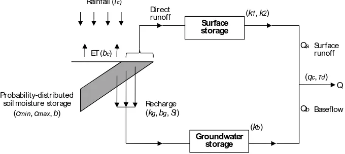
Fig. 3. Conceptual structure of the PDM model. The 13 model parameters to be calibrated are in the brackets.

soil moisture conditions. The groundwater recharge is then routed through a “slow response system”, which can be best represented by a cubic form of a nonlinear storage model (Dooge, 1973). The direct flow, defined as the difference be-tween the soil moisture storage at the beginning and the end of a time interval, is routed through “a fast response system”, which is often described by a cascade of two linear reservoirs (O’Connor, 1982). Further details of the model equations are presented by Moore (2007). Figure 3 shows the conceptual structure of the PDM model. Table 2 lists the 13 parameters to be calibrated in the model.

2.2.2 The real-time updating scheme: ARMA

Error prediction is now a well-established technique for fore-cast updating in real time (Box and Jenkins, 1970; Moore, 1982). The real-time updating scheme used in this study is wholly external to the deterministic model operation and thus can be easily applied in combination with any kind of rainfall–runoff models. A feature of errors from a con-ceptual rainfall–runoff model is that there is a tendency for errors to persist so that sequences of positive errors (un-derestimation) or negative errors (overestimation) are com-mon (Moore, 2007). This dependent structure in the error se-quence may be exploited by developing an error predictor which incorporates the error structure and allows for future

errors to be predicted. In this updating scheme, the structure of errors is analysed and the predictions of future errors are added to the deterministic model prediction to obtain the up-dated and improved forecasts of flow. Withqt+lrepresenting

the modelling result of the observed flowQt+l at a certain

timet+l, directly obtained from the PDM model without in-corporating the observed flow data, the errorηt+l is defined

asQt+l−qt+l. Letηt+l|tdenote a prediction of the errorηt+l,

which is madelsteps ahead from a forecast origin at timet using an error predictor. Then a real-time forecast,qt+l|t, can

be expressed as the sum of the predicted error and the original modelling result:

qt+l|t =qt+l+ηt+l|t. (6)

Among various forms of error predictors, the ARMA model is considered to be most appropriate and parsimonious (Moore, 2007). The equations of the error predictionsηt+l|t

expressed by the ARMA model can be written as follows: ηt+l|t= −ϕ1ηt+l−1|t−ϕ2ηt+l−2|t− · · · −ϕpηt+l−p|t (7)

+θ1at+l−1|t+θ2at+l−2|t+ · · · +θqat+l−q|t l=1,2,·, s

,

whereϕ1, ϕ2,· · ·ϕpandθ1,θ2,· · ·θq are autoregressive and

moving-average parameters respectively, with

at+l−i|t =

0 l−i >0 at+l−i otherwise,

(7)

[image:7.595.111.486.82.228.2]

Table 2. Parameters in the PDM model (Moore, 2007).

Parameter Unit Suggested value Description

fc none 1 Rainfall factor

τd h 0 Time delay

cmin,cmax mm 0 Minimum and maximum soil moisture store capacity

b none 0.5 Exponent of the soil moisture distribution

be none 2.5 Exponent in the actual evaporation function

kg h mmbg−1 105 Groundwater recharge time constant

bg none 1.5 Exponent of the groundwater recharge function

St mm 0 Soil tension storage capacity in the recharge function

k1,k2 h 1–20 Time constants of the surface routing

kb h mm2 5–100 Time constant of the groundwater storage routing

qc m3s−1 0 Constant flow representing returns/abstractions

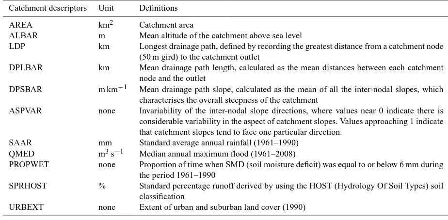
Table 3. Definitions of the FEH catchment descriptors (Bayliss, 1999).

Catchment descriptors Unit Definitions

AREA km2 Catchment area

ALBAR m Mean altitude of the catchment above sea level

LDP km Longest drainage path, defined by recording the greatest distance from a catchment node

(50 m gird) to the catchment outlet

DPLBAR km Mean drainage path length, calculated as the mean distances between each catchment

node and the outlet

DPSBAR m km−1 Mean drainage path slope, calculated as the mean of all the inter-nodal slopes, which

characterises the overall steepness of the catchment

ASPVAR none Invariability of the inter-nodal slope directions, where values near 0 indicate there is

considerable variability in the aspect of catchment slopes. Values approaching 1 indicate that catchment slopes tend to face one particular direction.

SAAR mm Standard average annual rainfall (1961–1990)

QMED m3s−1 Median annual maximum flood (1961–2008)

PROPWET none Proportion of time when SMD (soil moisture deficit) was equal to or below 6 mm during

the period 1961–1990

SPRHOST % Standard percentage runoff derived by using the HOST (Hydrology Of Soil Types) soil

classification

URBEXT none Extent of urban and suburban land cover (1990)

andat+l−i is the one-step ahead prediction error defined as

at+l−i≡at+l−i|t+l−i−1=ηt+l−i−ηt+l−i|t+l−i−1 (9) =Qt+l−i−qt+l−i|t+l−i−1

and

ηt+l−i|t=ηt+l−i=Qt+l−i−qt+l−i forl−i≤0. (10)

Equation (7) together with the related Eqs. (8–10) is used recursively to produce the error predictions ofηt+1|t,ηt+2|t,

· · ·,ηt+l|t, from the available values ofat,at−1,· · · andηt,

ηt−1,· · ·. Using this error prediction methodology, the PDM model original modelling results,qt+l, can be updated using

the error predictionηt+l|t, to calculate the required real-time

forecast,qt+l|t, according to Eq. (6).

As for the number of parameters in the ARMA structure, i.e.ϕ1,ϕ2,· · ·ϕpandθ1,θ2,· · ·θpin Eq. (7), a third-order

au-toregressive with dependence on three past model errors has

been proved to be an appropriate choice for UK conditions (Moore, 2007). Thus the ARMA structure containing three autoregressive parameters and one moving-average parame-ters (withp=3 andq=1) is chosen as the updating scheme in this study. It should be noted that for the forecasts made from an origint, by calculating the error predictorηt+l|t, the

real-time observations of flow are assimilated into the fore-casting results. For instance, with the structure of ARMA (3, 1), the observed flows att,t−1 andt−2 are involved in the calculation of the error predictorηt+l|t, which are then

added to the original model predictionqt+l to derive the

up-dated result ofqt+l|taccording to Eq. (6). For the obtaining of

qt+l, we assume the perfect knowledge of the future rainfall

[image:7.595.64.526.265.492.2]

(8)

39

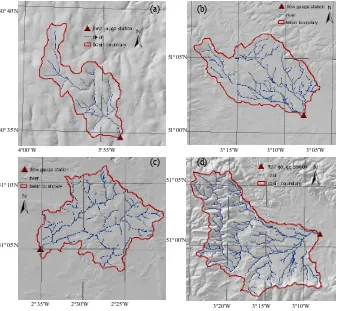
Figure 4 Locations and configurations of the four UK catchments in case studies with river networks and the flow gauging stations at the catchment outlets: (a) Bellever, (b) Halsewater, (c) Brue and (d) Bishop_Hull.

4°00′W 3°55′W 50°35′N

50°40′N (a)

51°05′N

51°00′N

3°10′W 3°05′W 3°15′W

(b)

3°20′W 3°15′W 3°10′W

51°05′N

51°00′N

(d)

2°35′W 2°30′W 2°25′W 51°10′N

51°05′N

[image:8.595.130.467.64.375.2]

(c)

Fig. 4. Locations and configurations of the four UK catchments in case studies with river networks and the flow gauging stations at the

catchment outlets (a) Bellever, (b) Halsewater, (c) Brue and (d) Bishop_Hull.

Table 4. Flow gauge locations and values of the FEH catchment descriptors for the four catchments in the case studies.

(A) (B) (C) (D)

Bellever Halsewater Brue Bishop_Hull

Flow gauge location Latitude 50.582◦N 51.022◦N 51.075◦N 51.019◦N

Longitude 3.898◦W 3.133◦W 2.587◦W 3.134◦W

Catchment

AREA (km2) 21.5 87.8 135.2 202.0

descriptors

ALBAR (m) 459 109 104 144

LDP (km) 13.46 19.40 22.61 40.21

DPLBAR (km) 6.28 9.57 13.62 17.75

DPSBAR (m km−1) 94.9 85.7 71.1 98.0

ASPVAR 0.25 0.30 0.16 0.17

SAAR (mm) 2095 851 857 964

QMED (m3s−1) 37.4 12.2 36.2 43.7

PROPWET 0.46 0.35 0.37 0.36

SPRHOST (%) 47.5 30.6 36.4 32.9

URBEXT 0 0.006 0.007 0.007

An automatic calibration procedure utilising an efficient population-based evolutionary optimisation technique, i.e. the particle swarm optimisation (PSO) algorithm (Eberhart and Kennedy, 1995, 2001), is adopted to estimate the four

[image:8.595.109.487.441.627.2]

(9)

2.3 Case study descriptions

2.3.1 Study catchments

Four catchments are selected from South West England, i.e. Bellever, Halsewater, Brue and Bishop_Hull, to carry out the case studies based on the constructed real-time forecasting system. They have different sizes of the drainage areas, vary-ing from 20 to 200 km2, as shown in Fig. 4. Except for the Bellever catchment, which is in the Devon area, with a maxi-mum altitude of 604 m above sea level, the other three catch-ments are located in the area of North Wessex, with an aver-age altitude of 119 m. All the catchments are predominantly rural areas with the main land-use types being the moorland, low-grade agriculture or woodland. Catchment descriptors are obtained from the Flood Estimation Handbook (FEH) (Bayliss, 1999) produced by the Centre of Ecology and Hy-drology (CEH) in the UK. Meanings of the descriptors are explained in Table 3, and values of the respective descrip-tors for the four catchments are listed in Table 4. It can be seen from Table 4 that the average annual rainfall (SAAR) is 2095 mm for the Bellever catchment with the percent-age runoff (SPRHOST) being 47.5 %, while the other three catchments have less rainfall (about 850–1000 mm per year) and slightly lower percentage runoff, i.e. 30.6 %, 36.4 % and 32.9 %. From the descriptors of the catchment size and con-figuration, it can be noticed that the increase of the catch-ment area (AREA) corresponds to an increase of LDP and DPLBAR, representing the longest and average length of the drainage path, which thus suggests an increasing travel time of the streamflow before it routes to the catchment outlet.

2.3.2 Data used in the case studies

Seven years of rainfall–runoff data are collected from the four catchments with a sampling interval of 15 min. The pe-riod is from October 1998 to September 2005 for Bellever, Halsewater and Bishop_Hull. Data from the HYREX (Hy-drological Radar Experiment) project funded by the NERC (Natural Environment Research Council) are used for the Brue catchment from September 1993 to May 2000. All the data are downsampled into other sequences with time inter-vals of 30, 45, 60, 90 and 120 min. Daily potential evapora-tion data are obtained from the MOSES and then disaggre-gated into the same time steps as the rainfall.

For each catchment, 1 yr data are selected for the valida-tion of the calibrated parameters of the rainfall–runoff model and the real-time updating scheme. Another 1 yr is used for independent evaluation of the model performance (i.e. the forecast accuracy). The remaining data of nearly five years are used for calibration. It is widely accepted that the infor-mation quality of the calibration data (i.e. the representative-ness of the catchment’s hydrological responses) is of more importance in deciding the performance of the calibrated model than the data length (Gupta and Sorooshian, 1985a, b).

According to the conclusions of Liu and Han (2010), a cali-bration dataset of 12 months contains sufficient information of hydrological variability to result in a reliable and stable model in the Brue catchment. In order to reduce the burden of the calculation work and improve the efficiency of data utilisation, in this study the most appropriate 1 yr data are se-lected from the calibration datasets for calibration using an effective selection index called the information cost function (ICF). More detailed information of the ICF index can be found in the work of Liu and Han (2010).

The 5 yr calibration data are first split into a group of cali-bration scenarios with the fixed length of 12 months, using a moving window of one month. As a result, up to 50 calibra-tion scenarios are resulted for each catchment. With the 1 yr validation data determined beforehand, the ICF index is used to select the most appropriate 10 calibration scenarios with sufficient hydrological information for calibration. Since the ICF index can only identify the relatively better calibration scenarios and not the absolutely best one, the 10 scenarios initially selected by ICF are used to carry out the calibration procedure. The best three calibrated models which have the best performances on the validation data are chosen to per-form the real-time forecasting 1–12 h ahead using the test-ing data, an independent 1 yr dataset of the calibration and validation data. Finally, the forecasting performances of the best three models are averaged. This is to present more sta-ble results, and in that way the uncertainty of calibration data, which is unavoidable in practice, can be involved in the final results.

It should be mentioned that the whole process described above is carried out for all the four catchments and repeated using data with different time intervals of 15, 30, 45, 60, 90 and 120 min. That is to say, for each data sequence with a cer-tain time interval, the calibration and validation procedures are carried out to construct a forecasting system that is suit-able to use with future data of the same time interval, and the real-time forecasting is made with the constructed sys-tem functioning at the same time step.

3 Results and discussion

3.1 Spectral differences of rainfall–runoff data with different time intervals

(10)

[image:10.595.90.509.94.293.2]

Table 5. Energy distributions in different frequency bands for 1 yr rainfall–runoff observations with different sampling intervals of 15, 30,

45, 60, 90 and 120 min.

Approx. Details Total energy

level 6 level 5 level 4 level 3 level 2 level 1

Frequency band [0, 9] [9, 17] [17, 35] [35, 69] [69, 139] [139, 278] [278, 566] [0, 566]

(10−6Hz)

flow

15 min 356 196 18 422 6848 543 39 3 1 382 052

30 min 356 176 18 375 6795 529 35 2 1 381 913

45 min 356 115 18 298 6705 504 29 2 1 381 654

60 min 356 026 18 175 6573 471 22 2 2 381 271

90 min 355 880 17 892 6253 395 18 7 2 380 447

120 min 355 718 17 477 5804 311 35 6 2 379 353

rain

15 min 112 56 71 80 86 78 43 526

30 min 112 56 71 77 73 41 30 460

45 min 112 56 70 71 57 33 16 415

60 min 112 55 68 66 50 15 13 379

90 min 112 55 63 50 29 8 10 327

120 min 112 54 59 42 18 7 7 299

Note: the observed data are taken from the Brue catchment of the UK with a sampling interval of 15 min. Four-year rainfall–runoff data

(19 September 1993 to 19 July 1997) are used to form 47 sets of 1 yr data with a moving window of one month. With the data collection methods of streamflow and rainfall described by Eqs. (1) and (2), each dataset is downsampled into another five series with time intervals of 30, 45, 60, 90 and 120 min. For a comparable analysis and a convenient calculation of the wavelet decomposition, extra data are added into the 30, 45, 60, 90 and 120 min data series in order to make them have the same amount of data as the 15 min series by either using a simple linear interpolation for the streamflow series or interpolating constant values for the rainfall. In such a case, all the data series have the same sampling interval of 15 min, and thus a sampling frequency of 1/900 Hz. The 47 pairs of data series of streamflow and rainfall with a certain time interval are used to perform the wavelet decomposition on 6 levels, which refer to the frequency bands of [278, 566]×10−6Hz, [139, 278]×10−6Hz, [69, 139]×10−6Hz, [35, 69]×10−6Hz, [17, 35]×10−6_{Hz and [9, 17]}_×₁₀−6_{Hz from level 1 to level 6. Finally, the decomposition results are averaged for the 47 pairs of data series with a certain}

time interval, and the energy values are calculated for each frequency band based on the wavelet coefficients.

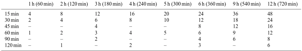
Table 6. Lead steps of the forecasting system with different time intervals.

1 h (60 min) 2 h (120 min) 3 h (180 min) 4 h (240 min) 5 h (300 min) 6 h (360 min) 9 h (540 min) 12 h (720 min)

15 min 4 8 12 16 20 24 36 48

30 min 2 4 6 8 10 12 18 24

45 min – – 4 – – 8 12 16

60 min 1 2 3 4 5 6 9 12

90 min – – 2 – – 4 6 8

120 min – 1 – 2 – 3 – 6

have very similar patterns, only those from the Daubechies wavelet of order 20 are presented.

The energies shown in Table 5 can be interpreted as the magnitudes of information content of the 1 yr data in differ-ent frequency bands. For the flow, the majority of energy is distributed in the lower bands, with little energy in the higher bands of level 1 to level 4. As for the rainfall, the energy dis-tribution is relatively balanced, with considerable amounts in all frequency bands. It has been pointed out by some studies (Bras, 1979; Bras and Rodriguez-Iturbe, 1976; Storm, 1989) that the catchment behaves like a low-pass filter to the cli-matic input data, e.g. rainfall and evapotranspiration, by ab-sorbing their subtle time variability. To further investigate the energy variance in a certain frequency band caused by the flow and rainfall data with different time intervals, it can be noticed that the variances for the flow series are not

ob-vious, considering the relatively large amounts of the total energies; however, with respect to the rainfall, the variances are more outstanding, which are on an increasing trend from the approximation to lower decomposition levels. In the low-frequency band of [0, 35×10−6_{] Hz (approximation + level} 6 + level 5), where most of the energy of the flow data is distributed, the energy variance of the rainfall series is less obvious compared to that in higher frequency bands. More-over, the energies of approximations are exactly the same for all the rainfall series. The difference of energy distribution for the flow and rainfall data with different intervals might be caused by the intrinsic characteristics of the two differ-ent hydrological processes, and also the differdiffer-ent sampling methods.

[image:10.595.56.540.416.498.2]

(11)

40 (a) Bellever

(Nov 2001~Apr 2002)

0 20 40 60 Flo w ( m 3/s ) 0 6 12 18 R a in fa ll ( m m /3 0 m in ) Observed Forecasted (b) Halsewater

(Nov 2001~Apr 2002)

0 20 40 60 Flo w ( m 3/s) 0 6 12 18 Ra in fa ll (m m /30 m in) Observed Forecasted (d) Bishop_Hull

(Nov 2001~Apr 2002)

0 20 40 60 Fl o w ( m 3/s) 0 6 12 18 R a in fa ll ( m m/ 3 0 min ) Observed Forecasted (c) Brue

(Nov 1999~Apr 2000)

0 20 40 60 Flo w ( m 3/s) 0 6 12 18 R a in fa ll ( mm/ 3 0 mi n ) Observed Forecasted

Figure 5 Six-month length hydrographs of the observed rainfall-runoff data versus the best results of the 4h-ahead forecasts using the 30 min data. The NSE values calculated between the observed and the forecasted flows are 0.8932, 0.9544, 0.9167 and 0.9420 respectively for the four catchments in subfigures (a), (b), (c) and (d).

Fig. 5. Six-month length hydrographs of the observed rainfall–runoff data versus the best results of the 4 h ahead forecasts using the 30 min

data. The NSE values calculated between the observed and the forecasted flows are 0.8932, 0.9544, 0.9167 and 0.9420 respectively for the four catchments in (a), (b), (c) and (d).

absorbed by the soil moisture reservoirs in the rainfall–runoff model (Oudin et al., 2004). As a consequence, the infor-mation content of the rainfall input in the higher frequency bands, which can show large variances with regard to a differ-ent time interval, is not likely to be transformed into the sim-ulated flow through the rainfall–runoff model. As discussed above, since the energy variances of the rainfall data in low frequency bands are not obvious, the transformed flow will not have much difference when using rainfall data with dif-ferent intervals as the input of the rainfall–runoff model. This indicates that the increased sampling rate for the rainfall data may not necessarily improve the performance of the rainfall– runoff model. This has been verified by many studies; for ex-ample, Schaake et al. (1996) found that using 6 h, 12 h, 1-day, 2-day and 4-day rainfall data could generate similar simula-tion results of flow as long as the model was calibrated and operated at the same time intervals. However, this conclusion may only be true for pure simulation using the rainfall–runoff model. The energy distribution from the wavelet analysis is not enough to provide a general pattern for the impact of time interval on real-time forecasting, where the existence of the real-time updating scheme involves the historical flow data as another system input together with the rainfall. In the fol-lowing sections, the impact of data time interval in real-time hydrological forecasting is explored through the case studies.

3.2 Relation between the optimal time interval and the

forecast lead time

For the four catchments in the case studies, the following analyses of data time interval are based on the performances of the real-time forecasting system on the respective 1 yr test-ing data with lead times of 1–6, 9 and 12 h. The lead steps of the forecasting system constructed from data with different time intervals are shown in Table 6. It can be noticed that for some forecast lead times such as 1, 2, 3, 4, 5 and 9 h, there are no integers for the time intervals of 45, 90 and 120 min. Therefore, forecasts are not made for such lead times by the forecasting systems constructed from the 45, 90 and 120 min data.

(12)

[image:12.595.129.465.94.489.2]

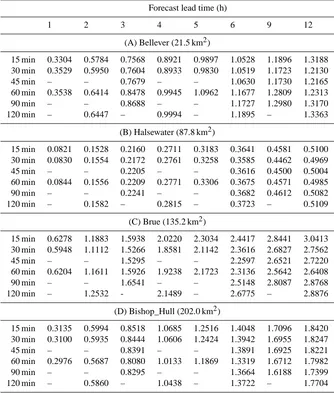
Table 7. Forecasting results shown in RMSE (m3s−1) for the four catchments using data with different time intervals. The lowest RMSE

value for a certain lead time is highlighted to show the optimal data time interval.

Forecast lead time (h)

1 2 3 4 5 6 9 12

(A) Bellever (21.5 km2)

15 min 0.2099 0.4870 0.7232 0.8915 1.0039 1.0754 1.1530 1.1593

30 min 0.2359 0.4851 0.6699 0.7955 0.8801 0.9378 1.0200 1.0448

45 min – – 0.6754 – – 0.9218 0.9981 1.0231

60 min 0.2938 0.5359 0.7073 0.8175 0.8907 0.9401 1.0143 1.0395

90 min – – 0.7942 – – 1.0489 1.1083 1.1260

120 min – 0.5833 – 0.9042 – 1.0189 – 1.0832

(B) Halsewater (87.8 km2)

15 min 0.0555 0.1177 0.1859 0.2516 0.3111 0.3638 0.4863 0.5672

30 min 0.0570 0.1211 0.1883 0.2510 0.3061 0.3535 0.4585 0.5238

45 min – – 0.1896 – – 0.3626 0.4827 0.5635

60 min 0.0605 0.1243 0.1930 0.2578 0.3161 0.3668 0.4842 0.5623

90 min – – 0.1905 – – 0.3644 0.4802 0.5568

120 min – 0.1246 – 0.2600 – 0.3668 – 0.5441

(C) Brue (135.2 km2)

15 min 0.2641 0.7190 1.1873 1.5767 1.8617 2.0583 2.3422 2.3939

30 min 0.3172 0.7824 1.2185 1.5671 1.8263 2.0157 2.3155 2.3867

45 min – – 1.2121 – – 1.9803 2.2150 2.2654

60 min 0.3208 0.8044 1.2549 1.5896 1.8114 1.9554 2.1539 2.1984

90 min – – 1.2584 – – 1.9229 2.0934 2.1395

120 min – 0.9306 – 1.7574 – 2.1469 – 2.3157

(D) Bishop_Hull (202.0 km2)

15 min 0.1496 0.3849 0.6502 0.9099 1.1468 1.3567 1.8314 2.1099

30 min 0.1447 0.3677 0.6210 0.8713 1.1007 1.3048 1.7792 2.0676

45 min – – 0.7068 - - 1.4327 1.8736 2.1137

60 min 0.1644 0.4088 0.6783 0.9291 1.1436 1.3213 1.6848 1.8869

90 min – – 0.7190 – – 1.3865 1.7814 2.0101

120 min – 0.4576 – 0.9703 – 1.3422 – 1.8412

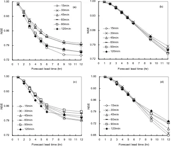
and the forecast lead time are on decreasing trends. When comparing the differences between the six curves, it can be found that as the lead time increases, the distance of the curves becomes increasingly larger until finally the curves are clearly distinct from each other. This means that when the lead time is small, e.g. from 1 to 6 h, the variance of the fore-casts resulted from data with different time intervals is also subtle, while with the increase of the lead time, e.g. when exceeding 6 hours, the variance becomes more and more sig-nificant. This proves that the choice of the time interval does have a considerable impact on the forecasting results, which is even more prominent with longer forecast lead times than shorter ones.

The lowest RMSE values for the forecasts made with a cer-tain lead time are highlighted in Table 7 to show the optimal choice of the time interval for a certain lead time forecast. It can be seen that there is an increase of the optimal time

(13)

41

(a)

0.72 0.79 0.86 0.93 1.00

0 1 2 3 4 5 6 7 8 9 10 11 12

Forecast lead time (hr)

NS

E

15min

30min

45min

60min 90min

120min

(b)

0.72 0.79 0.86 0.93 1.00

0 1 2 3 4 5 6 7 8 9 10 11 12

NS

E 15min

30min

45min

60min 90min

120min

(c)

0.72 0.79 0.86 0.93 1.00

0 1 2 3 4 5 6 7 8 9 10 11 12

NS

E

15min

30min 45min

60min

90min

120min

(d)

0.65 0.72 0.79 0.86 0.93 1.00

0 1 2 3 4 5 6 7 8 9 10 11 12

NS

E _15min

30min

45min

60min

90min

120min

Figure 6 Decreasing performance of the forecasting system constructed using data with

[image:13.595.128.468.65.358.2]

different time intervals as the increase of the forecast lead time, for the catchments of Bellever, Halsewater, Brue and Bishop_Hull, respectively in (a), (b), (c) and (d).

Fig. 6. Decreasing performance of the forecasting system constructed using data with different time intervals with the increase of the forecast

lead time, for the catchments of Bellever, Halsewater, Brue and Bishop_Hull, respectively in (a), (b), (c) and (d).

simply building the model using data as they are originally measured.

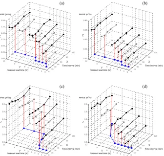
To make the patterns shown by Table 7 more obvious, the forecasting results are plotted in three-dimensional co-ordinates for the four catchments, as shown in Fig. 7. The x axis stands for the data time interval (15, 30, 45, 60, 90 and 120 min); the y axis represents the eight forecast lead times (1, 2, 3, 4, 5, 6, 9, 12 h); and the values on the vertical zaxis show the forecasting results in RMSE. In each subfig-ure, each of the eight suspended curves indicates the variance of the forecast accuracy with respect to different time inter-vals for forecasts made with a certain lead time. The lowest points of the eight curves (representing the optimal time in-tervals which result in the least forecasting errors) are pro-jected onto thex-y plane and then connected together. The projection curve (in blue) thus reveals the relationship be-tween the optimal time interval and the forecast lead time. It can be seen that all the four projection curves for the four catchments are on increasing trends, which indicates the in-crease of the optimal time interval with the inin-crease of the forecast lead time. This is consistent with the previous con-clusions made by examining the rankings in Table 8. How-ever, besides the positive relation between the optimal time interval and the forecast lead time, it can also be noted that the increasing patterns of the projection curves are quite

dif-ferent for the four catchments. The reason for these various increasing patterns will be fully discussed in the next section.

3.3 Implications of the catchment concentration time

(14)

3652 J. Liu and D. Han: Optimal data time interval for real-time hydrological forecasting 42 0 15 30 45 60 90 120 0 1 2 3 4 5 6 9 12 0.00 0.25 0.50 0.75 1.00 1.25 1.50 X Y Z 0 15 30 45 60 90 120 0 1 2 3 4 5 6 9 12 0.00 0.20 0.40 0.60 0.80 X Y Z 0 15 30 45 60 90 120 0 1 2 3 4 5 6 9 12 0.0 0.5 1.0 1.5 2.0 2.5 X Y Z 0 15 30 45 60 90 120 0 1 2 3 4 5 6 9 12 0.0 0.5 1.0 1.5 2.0 2.5 X Y Z

Figure 7 Forecasting results in three-dimensional coordinates for the four catchments, of Bellever, Halsewater, Brue and Bishop_Hull, respectively in subfigures (a), (b), (c) and (d).

(a) (b)

(c) (d)

Forecast lead time (hr) RMSE (m3

/s)

Time interval (min) Time interval (min)

RMSE (m3 /s)

RMSE (m3

/s) RMSE (m3

/s)

[image:14.595.132.469.62.381.2]

Fig. 7. Forecasting results in three-dimensional coordinates for the four catchments, of Bellever, Halsewater, Brue and Bishop_Hull,

respec-tively in (a), (b), (c) and (d).

representing a lower catchment steepness, which thus indi-cates a longer concentration time compared to Bellever. All these facts imply that a longer concentration time might re-sult in a sharper increase of the projection curve, while on the other hand, a flatter curve might be resulted from a catchment with a quicker response.

FEH provides a simple method to calculate the catchment concentration time using a generalised model of the catch-ment descriptors derived by regression analysis (Houghton-Carr, 1999), as shown by Eq. (11):

Tp=4.270×DPSBAR−0.35×PROPWET−0.80× (11) DPLBAR0.54×(1+URBEXT)−5.77

,

whereTp stands for the time to peak of the instantaneous unit hydrograph. The advantage of this equation is that it is theoretically independent of the time interval, which enables an independent evaluation of catchment concentration time other than those normally derived by using rainfall–runoff data sampled with a certain time interval (Littlewood and Croke, 2008). The calculated results of the four catchments are 4.36, 6.81, 8.37 and 8.82 h, respectively for Bellever, Halsewater, Brue and Bishop_Hull. This is in agreement with the above conclusion made by simply examining the values

of the catchment descriptors of LDP, DPLBAR and DPS-BAR. It should be mentioned that results from the Eq. (11) also can only provide a provisional comparison of the con-centration times, which may not be treated as the realistic response times of the catchment (Houghton-Carr, 1999).

(15)

Table 8. Rankings of different time intervals according to the

fore-casting results (RMSE) with a certain lead time (from the lowest to the highest RMSE). The optimal time intervals (ranked as the 1st) are highlighted.

1 h 2 h 3 h 4 h 5 h 6 h 9 h 12 h

1st 15 30 30 30 30 45 45 45

2nd 30 15 45 60 60 30 60 60

3rd 60 60 60 15 15 60 30 30

4th – 120 15 120 – 90 90 120

5th – – 90 – – 120 15 90

6th – – – – – 15 – 15

optimal 15 30 30 30 30 45 45 45

1st 15 15 15 30 30 30 30 30

2nd 30 30 30 15 15 45 90 120

3rd 60 60 45 60 60 15 45 90

4th – 120 60 120 – 90 60 60

5th – – 90 – – 60 15 45

6th – – – – – 120 – 15

optimal 15 15 15 30 30 30 30 30

(C) Brue (135.2 km2)

1st 15 15 15 30 60 90 90 90

2nd 30 30 45 15 30 60 60 60

3rd 60 60 30 60 15 45 45 45

4th – 120 60 120 – 30 30 120

5th – – 90 – – 15 15 30

6th – – – – – 120 – 15

optimal 15 15 15 30 60 90 90 90

1st 30 30 30 30 30 30 60 120

2nd 15 15 15 15 60 60 30 60

3rd 60 60 60 60 15 120 90 90

4th – 120 45 120 – 15 15 30

5th – – 90 – – 90 45 15

6th – – – – – 45 – 45

optimal 30 30 30 30 30 30 60 120

All the above analyses indicate that the concentration time might play a considerable role in influencing the selection of the optimal time interval when the forecast lead time is determined. It is known that a steeper, naturally wetter and more urbanised catchment tends to have a faster response, while the larger and longer the catchment is, the slower the response will be. However, besides the descriptors presented in Table 3 and used in Eq. (11), the concentration time is also affected by many other factors (Akan, 1989), e.g. the density of the watercourse, the consistency of the flow directions, the soil infiltration conditions, the rainfall intensity and the storm

path, etc. As a consequence, although it can be deduced from the above analyses that the longer the concentration time is, the steeper the projection curve tends to be, the various in-fluencing factors make it difficult to figure out how exactly the selection of the optimal time interval is affected by the concentration time. And it is far too early to say that the con-centration time is definitely the principal factor determining the increasing pattern of the optimal time interval with re-spect to the increase of the forecast lead time. More research with various catchments bearing different response charac-teristics is needed to explore the underlying factors and their functions in determining the optimal time interval.

3.4 A hypothetical pattern for the selection of the optimal time interval

Based on the analyses of the forecasting results in the case studies, it is interesting to note that the conclusions from the four catchments are consistent with the findings in modern control engineering as mentioned in the introduction part; that is, the best forecasts with a certain lead time are not al-ways produced by the finest time interval or the largest one. Conversely, in hydrological forecasting, the optimal choice of the time interval is found to be increased with the exten-sion of the forecast lead time. Following this, a generalised pattern for the selection of the optimal time interval in real-time hydrological forecasting can be proposed, as shown in Fig. 8, in similar three-dimensional coordinates as Fig. 7.

In Fig. 8, thex,y andzaxes represent the time interval, the forecast lead time and the forecasting error in the three subfigures respectively. Two U-shape curves are used to de-scribe the relations between the forecasting error and the time interval in two cases when forecasts are made with a small forecast lead time and a long lead time, as shown respec-tively in Fig. 8a and b. The lowest points of the two U-shape curves, (X1,Z1) and (XN,ZN) thus represent the optimal

choices of the time interval in the two cases. As concluded from the case studies, with the increase of the forecast lead time, the forecasting accuracy is decreasing and the optimal time interval is on an increase. Consequently, the two low-est points have the relations ofZ1< ZNandX1< XN. This

(16)

[image:16.595.130.464.96.489.2]

Table 9. Forecasting results shown in RMSE (m3s−1) for the four catchments using data with different time intervals: similar to Table 7 but without updating of the ARMA model. The lowest RMSE value for a certain lead time is highlighted to show the optimal data time interval.

Forecast lead time (h)

1 2 3 4 5 6 9 12

15 min 0.3304 0.5784 0.7568 0.8921 0.9897 1.0528 1.1896 1.3188

30 min 0.3529 0.5950 0.7604 0.8933 0.9830 1.0519 1.1723 1.2130

45 min – – 0.7679 – – 1.0630 1.1730 1.2165

60 min 0.3538 0.6414 0.8478 0.9945 1.0962 1.1677 1.2809 1.2313

90 min – – 0.8688 – – 1.1727 1.2980 1.3170

120 min – 0.6447 – 0.9994 – 1.1895 – 1.3363

15 min 0.0821 0.1528 0.2160 0.2711 0.3183 0.3641 0.4581 0.5100

30 min 0.0830 0.1554 0.2172 0.2761 0.3258 0.3585 0.4462 0.4969

45 min – – 0.2205 – – 0.3616 0.4500 0.5004

60 min 0.0844 0.1556 0.2209 0.2771 0.3306 0.3675 0.4571 0.4985

90 min – – 0.2241 – – 0.3682 0.4612 0.5082

120 min – 0.1582 – 0.2815 – 0.3723 – 0.5109

(C) Brue (135.2 km2)

15 min 0.6278 1.1883 1.5938 2.0220 2.3034 2.4417 2.8441 3.0413

30 min 0.5948 1.1112 1.5266 1.8581 2.1142 2.3616 2.6827 2.7562

45 min – – 1.5295 – – 2.2597 2.6521 2.7220

60 min 0.6204 1.1611 1.5926 1.9238 2.1723 2.3136 2.5642 2.6408

90 min – – 1.6541 – – 2.5148 2.8087 2.8768

120 min – 1.2532 - 2.1489 – 2.6775 – 2.8876

15 min 0.3135 0.5994 0.8518 1.0685 1.2516 1.4048 1.7096 1.8420

30 min 0.3100 0.5935 0.8444 1.0606 1.2424 1.3942 1.6955 1.8247

45 min – – 0.8391 – – 1.3891 1.6925 1.8221

60 min 0.2976 0.5687 0.8080 1.0133 1.1869 1.3319 1.6712 1.7982

90 min – – 0.8295 – – 1.3664 1.6188 1.7399

120 min – 0.5860 – 1.0438 – 1.3722 – 1.7704

It should be emphasised that this hypothetical pattern of the optimal time interval is especially proposed for real-time forecasting, rather than simulation with only the rainfall– runoff model. When making forecasts using either the data-driven model (e.g. ANN and TF model, etc.) or the physically based rainfall–runoff model together with a real-time updat-ing scheme, an extrapolation is made based on the historical data and into the future. Too dense data will result in worse extrapolation further into the future, while too sparse data can also make the extrapolation fail in the very near future. In essence, this is why using different data time intervals makes a difference to the forecasting results. On the other hand, for the simulation mode using the rainfall–runoff model only, the simulated flow may not vary too much when different data time intervals are used. As analysed in Sect. 3.1, this is due to the low-pass-filtering function of the rainfall–runoff model, which filter out high-frequency variances of the rainfall data

with different time intervals as the input of the system. How-ever, in real-time forecasting, besides rainfall, the flow obser-vations are involved as another input of the modelling system through the updating scheme (e.g. the ARMA model). This can explain why the optimal time interval exists in real-time forecasting but not in the case of pure simulation, at least for those commonly used time intervals examined in this study. But it is believed that with an infinitely small or large time interval, modelling results in simulation mode can also de-teriorate due to the involvement of measurement noises or the lack of efficient representation of the original signals of rainfall.

(17)

43

X1

Z1

ZN

XN

Figure 8 Hypothetical pattern for the general impact of data time interval on forecasting

accuracy and the selection of the optimal time interval in real-time hydrological forecasting. The axes of X, Y and Z respectively stand for the time interval of the model input data, the forecast lead time and the forecasting error.

(a)

X Z

Y

X1

XN

YN

Y1

Z1

ZN

(c)

(b)

Fig. 8. Hypothetical pattern for the general impact of data time

in-terval on forecasting accuracy and the selection of the optimal time

interval in real-time hydrological forecasting. The axes ofX,Y and

Zrespectively stand for the time interval of the model input data,

the forecast lead time and the forecasting error.

As discussed above, the updating scheme is the most likely reason for the existence of the optimal time interval and its positive relation with the forecast lead time. It is interesting to see how much the current results depend on the updat-ing scheme, i.e. the ARMA model in this study. Table 9 lists the forecasting results of the four catchments using the same datasets and methodologies as described in the case studies, but without the real-time updating using the ARMA model. Instead, previous one-step errors are directly added to fore-casts of the future flow. It can be seen in Table 9 that there is an overall increase of the forecasting errors compared to the results with the use of the ARMA model (shown by Ta-ble 7). For a certain forecast lead time, the optimal time inter-vals still exist, and they show an increasing trend with the in-crease of the forecast lead time. However, the optimal values are not identical to those in Table 7. For a better comparison, the optimal time intervals are plotted in Fig. 9 against the forecast lead time in the two circumstances with and without the updating of ARMA. It can be found for each study catch-ment in Fig. 9 that the increasing pattern of the curve without ARMA updating is not as sharp as the ARMA one. These modest patterns indicate that the impacts of the data time interval are alleviated when the ARMA model is not used. However, it is still true that the increasing pattern is sharper for larger catchments without the use of ARMA; for exam-ple, the optimal time intervals for the 12 h lead time increase to 90, 60, 30 and 30 min for the catchments of Bishop_Hull, Brue, Halsewater and Bellever with a decreasing drainage area respectively. The results without the use of the ARMA model can be treated as a baseline to evaluate the impact of the data time interval when more complicated updating schemes are adopted in the forecasting system. Regarding the differences caused by using different updating schemes, it is important that more case studies are explored using different forecasting systems (i.e. combinations of different rainfall– runoff models with different updating schemes) in various

geographical and climatic regions. In such a case the pro-posed hypothetical pattern of the data time interval may be further verified and improved, or otherwise refuted; for ex-ample, is the pattern universal or only applicable to a certain types of forecasting systems and catchments?

Another question that deserves attention is the estimation of the catchment areal rainfall, which is regarded as one of most significant sources of uncertainty in hydrological fore-casting (Sene et al., 2009). In this study, the simplest linear weighting method, i.e. Thiessen polygons, is used to aver-age the rain gauge observations for the catchments. The four catchments have relatively small areas (20 to 200 km2) cov-ered by dense rain gauges. Take the Brue catchment, for ex-ample; it has 49 tipping-bucket rain gauges over the drainage area of 135.2 km2. Although the other three catchments have lower rain gauge densities, they show very similar patterns of the forecasting results to the Brue. In this case, the estimation of the catchment areal rainfall is not a major problem in this study. However, for large catchments with sparse rain gauge networks, the averaging methods may bring uncertainties in revealing the true patterns between the optimal data time interval and the forecast lead time. The question becomes broader in the combination of the spatial information of radar with the point observations of rain gauges, especially when the radar estimates of rainfall are involved (Cole and Moore, 2008, 2009). Besides the estimation of the areal rainfall, the error measurement statistics adopted to evaluate the perfor-mance of the forecasting system may also bring uncertainties into the study. Hall (2001) addressed the error measurement issue and analysed 10 commonly used indices to evaluate the goodness of fit of a model to a set of observations, and it was found that not a single error measurement method was per-fect. In this study, two square-error-based statistics, RMSE and NSE, were chosen considering their popularity in hydro-logical forecasting. However, other error evaluation methods are worth trying in order to attest to whether the hypotheti-cal pattern is limited to a certain type of error measurement statistics.

4 Conclusions

[image:17.595.51.285.63.195.2]

(18)

3656 J. Liu and D. Han: Optimal data time interval for real-time hydrological forecasting 44 (a) Bellever 0 15 30 45 60 75 90 105 120

1h 2h 3h 4h 5h 6h 9h 12h Forecast lead time

Ti m e i n te rv a l (m in ) ARMA

without ARMA (b) Halsewater

0 15 30 45 60 75 90 105 120

Ti m e i n te rv a l ( m in ) ARMA without ARMA (c) Brue 0 15 30 45 60 75 90 105 120

Ti m e i n te rv a l ( m in ) ARMA without ARMA (d) Bishop_Hull 0 15 30 45 60 75 90 105 120

Ti m e i n te rv a l ( m in ) ARMA without ARMA

Figure 9 Comparisons on the data time interval patterns when the real-time hydrological

[image:18.595.128.468.64.334.2]

forecasts are made in the two circumstances with/without the updating of the ARMA model.

Fig. 9. Comparisons on the data time interval patterns when the real-time hydrological forecasts are made in the two circumstances

with/without the updating of the ARMA model.

engineering, but is a largely ignored topic in the area of op-erational hydrological forecasting.

In the beginning of this study, discrete wavelet transform is used to examine the spectral variances of rainfall–runoff data with different time intervals in the frequency domain. It is found that the rainfall signal has energy spread more widely than the flow, but due to the low-pass-filtering func-tion of the rainfall–runoff model, the high-frequency vari-ances of the rainfall signal with different time intervals are not likely to be transformed into the flow. This indicates that higher sampling rates may not always help to improve the re-sults of rainfall–runoff modelling. To further investigate the impact of time interval in real-time hydrological forecasting, which becomes more complicated by involving the flow data as the system inputs by the updating scheme, case studies are carried out in four catchments with different drainage areas and concentration times. Main findings from the case studies can be concluded as follows: (1) the data time interval does have a considerable impact on the performance of the fore-casting system, which is more prominent to longer lead times than shorter ones; (2) there exists an optimal time interval for forecasts made with a certain lead time, and the length of the optimal time interval is increasing with the increase of the forecast lead time; (3) the positive relation between the opti-mal time interval and the forecast lead time can show various patterns, which is found to be highly related to the catchment concentration time; and (4) the longer the concentration time

is, the more dramatically the optimal time interval tends to increase with the increase of the forecast lead time. Finally, according to the results of the case studies, a hypothetical pattern is proposed in three-dimensional coordinates for the selection of the optimal time interval in real-time hydrologi-cal forecasting.