Testing the realism of a topography driven model (FLEX Topo) in the nested catchments of the Upper Heihe, China

Hydrol. Earth Syst. Sci., 18, 1895–1915, 2014 www.hydrol-earth-syst-sci.net/18/1895/2014/ doi:10.5194/hess-18-1895-2014

© Author(s) 2014. CC Attribution 3.0 License.

Testing the realism of a topography-driven model (FLEX-Topo)

in the nested catchments of the Upper Heihe, China

H. Gao1, M. Hrachowitz1, F. Fenicia1,2, S. Gharari1,3, and H. H. G. Savenije1 1_{Water Resources Section, Delft University of Technology, Delft, the Netherlands}

2_{Eawag: Swiss Federal Institute of Aquatic Science and Technology, Dübendorf, Switzerland}

3_{Department of Environment and Agro-Biotechnologies, Centre de Recherche Public – Gabriel Lippmann,} Belvaux, Luxembourg

Correspondence to: H. Gao ([email protected])

Received: 14 September 2013 – Published in Hydrol. Earth Syst. Sci. Discuss.: 22 October 2013 Revised: 25 February 2014 – Accepted: 8 April 2014 – Published: 22 May 2014

Abstract. Although elevation data are globally available and used in many existing hydrological models, their information content is still underexploited. Topography is closely related to geology, soil, climate and land cover. As a result, it may reflect the dominant hydrological processes in a catchment. In this study, we evaluated this hypothesis through four pro-gressively more complex conceptual rainfall-runoff models. The first model (FLEXL) is lumped, and it does not make use of elevation data. The second model (FLEXD_{) is} semi-distributed with different parameter sets for different units. This model uses elevation data indirectly, taking spatially variable drivers into account. The third model (FLEXT0), also semi-distributed, makes explicit use of topography in-formation. The structure of FLEXT0consists of four paral-lel components representing the distinct hydrological func-tion of different landscape elements. These elements were determined based on a topography-based landscape classi-fication approach. The fourth model (FLEXT) has the same model structure and parameterization as FLEXT0but uses re-alism constraints on parameters and fluxes. All models have been calibrated and validated at the catchment outlet. Addi-tionally, the models were evaluated at two sub-catchments. It was found that FLEXT0 and FLEXT perform better than the other models in nested sub-catchment validation and they are therefore better spatially transferable. Among these two models, FLEXTperforms better than FLEXT0in transferabil-ity. This supports the following hypotheses: (1) topography can be used as an integrated indicator to distinguish between landscape elements with different hydrological functions; (2) FLEXT0and FLEXTare much better equipped to represent

the heterogeneity of hydrological functions than a lumped or semi-distributed model, and hence they have a more realistic model structure and parameterization; (3) the soft data used to constrain the model parameters and fluxes in FLEXTare useful for improving model transferability. Most of the pre-cipitation on the forested hillslopes evaporates, thus generat-ing relatively little runoff.

1 Introduction

Topography plays an important role in controlling hydrolog-ical processes at catchment scale (Savenije, 2010). It may not only be a good first-order indicator of how water is routed through and released from a catchment (Knudsen et al., 1986), it also has considerable influence on the dom-inant hydrological processes in different parts of a catch-ment, which could be used to define hydrologically dif-ferent response units (Savenije, 2010). As an indicator for hydrological behaviour, topography is also linked to geol-ogy, soil characteristics, land cover and climate through co-evolution (Sivapalan, 2009; Savenije, 2010). Thus, informa-tion on other features can to some extent be inferred from to-pography. However, the information provided by topography is generally underexploited in hydrological models although it is, explicitly or implicitly, incorporated in many models (e.g. Beven and Kirkby, 1979; Knudsen, 1986; Uhlenbrook et al., 2004).

As a typical lumped topography-driven model, TOP-MODEL (Beven and Kirkby, 1979) uses the topographic

1896 H. Gao et al.: Testing the realism of a topography-driven model (FLEX-Topo) – Upper Heihe, China wetness index (TWI) (Beven and Kirkby, 1979), which is

a proxy for the probability of saturation of each point in a catchment, to consider the influence of topography on the occurrence of saturated overland flow (SOF). Simi-larly, the Xinanjiang model (Zhao, 1992) implicitly consid-ers the influence of topography in its soil moisture function, as the curve of its tension water capacity distribution can be interpreted as topographic heterogeneity. Conceptually, both models implicitly reflect the variable contributing area (VCA) concept. Although the topography-aided VCA repre-sentation is present in many models, experimental evidence has shown that its underlying assumptions may not always hold (Western et al., 1999; Spence and Woo, 2003; Tromp-van Meerveld and McDonnell, 2006). In view of these lim-itations, and in spite of their often demonstrated suitability, there is an urgent need to explore new and potentially more generally applicable ways to incorporate topographic infor-mation in conceptual hydrological models.

Other types of topographically driven hydrological models are distributed physically based models, which use topogra-phy essentially to define flow gradients and flow paths of wa-ter (Refsgaard and Knudsen, 1996). The limitations of this kind of “bottom-up” model approach include the increased computational cost, and maybe more importantly, the unac-counted scale effects (Abbott and Refsgaard, 1996; Beven and Germann, 2013; Hrachowitz et al., 2013b). Knudsen et al. (1986) developed a semi-distributed, physically based model, which divides the whole catchment into several dis-tinct hydrological response units defined by the catchment characteristics such as meteorological conditions, topogra-phy, vegetation and soil types. Although this type of model was shown to work well in case studies, approaches like this suffer from their intensive data requirement and complex model structure, similar to modelling approaches based on the dominant runoff process concept (Grayson and Blöschl, 2001; Scherrer and Naef, 2003). The main problem with physically based models appears to be that by breaking up catchments into small interacting cells, patterns present in the landscape are broken up as well. The question is how to make use of landscape diversity, and the related hydrologi-cal processes, while maintaining the larger shydrologi-cale patterns and without introducing excessive complexity.

The recently suggested topography-driven conceptual modelling approach (FLEX-Topo) (Savenije, 2010), which attempts to exploit topographic signatures to design concep-tual model structures as a means to find the simplest way to represent the complexity and heterogeneity of hydrolog-ical processes, forms a middle way between parsimonious lumped and complex distributed models, and represents the subject of this study. In the framework of FLEX-Topo, to-pographic information is regarded as the main indicator of landscape classes and dominant hydrological processes. A valuable key for hydrologically meaningful landscape clas-sification is the recently introduced metric HAND (Height Above the Nearest Drainage) (Rennó et al., 2008; Nobre et

al., 2011; Gharari et al., 2011), which is a direct reflection of hydraulic head to the nearest drain. Consequently, within a flexible modelling framework (Fenicia et al., 2008, 2011), different model structures can be developed to represent the different dominant hydrological processes in different land-scape classes. Note that FLEX-Topo is not another concep-tual model but rather a modelling framework to make more exhaustive use of topographic information in hydrological models and it can in principal be applied to any type of con-ceptual model.

Model transferability is one of the important indicators in testing model realism (Klemeš, 1986). Although many hy-drological models, both lumped and distributed, frequently perform well in calibration, transferring them and their pa-rameter sets into other catchments, or even into nested sub-catchments, remains problematic (Pokhrel and Gupta, 2011). There are several reasons for this: uncertainty in the data, in-sufficient information provided by the hydrograph or an un-suitable model structure which does not represent the dom-inant hydrological processes or their spatial heterogeneity sufficiently well (Gupta et al., 2008). Various techniques to improve model transferability have been suggested in the past (Seibert and McDonnell, 2002; Uhlenbrook and Lei-bundgut, 2002; Khu et al., 2008; Hrachowitz et al., 2013b; Euser et al., 2013; Gharari et al., 2013b), and it became clear that successful transferability critically depends on appropri-ate methods to link catchment characteristics to model struc-tures and parameters or in other words to link catchment form to hydrological function (Gupta et al., 2008).

H. Gao et al.: Testing the realism of a topography-driven model (FLEX-Topo) – Upper Heihe, China 1897

27

Table 9. The simulated results of FLEX

1

Bare soil/rock (18%) Forest hillslope (17%) Grassland hillslope (31%) Wetland/Terrace (36%)

P (mm/a) 481 P (mm/a) 431 P (mm/a) 431 P (mm/a) 410

EaB (mm/a) 174 EiFH (mm/a) 125 EiGH (mm/a) 58 EiW (mm/a) 87 RpB (mm/a) 115 EaFH (mm/a) 257 EaGH (mm/a) 205 EaW (mm/a) 220 RrB (mm/a) 107 RsFH (mm/a) 15 RsGH (mm/a) 63 CR (mm/a) 21 QffB (mm/a) 77 QfFH (mm/a) 26 QfGH (mm/a) 101 QrW (mm/a) 122

2

3

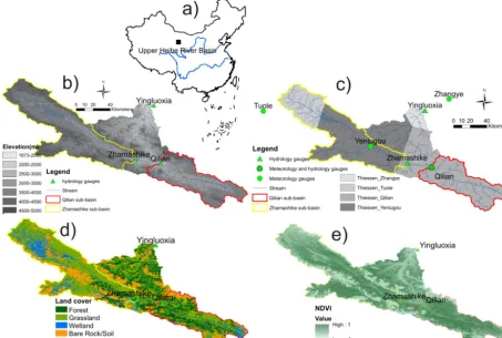
Fig.1. (a) location of the Upper Heihe in China; (b) DEM of the Upper Heihe with its runoff

4

gauging stations, meteorological stations, streams and the outline of two sub-catchments; (c)

5

meteorological stations and associated Thiessen polygons, the different grayscale indicates

6

different long term annual average precipitation (the darker the more precipitation: Zhangye

7

is 131 (mm/a); Tuole is 293 (mm/a); Qilian is 394 (mm/a); Yeniugou is 413(mm/a)); (d) land

8

cover map of the Upper Heihe; (e) averaged NDVI map in the summer of 2002.

9

10

11

Figure 1. (a) Location of the Upper Heihe in China; (b) DEM of the Upper Heihe with its runoff-gauging stations, meteorological stations, streams and the outline of two sub-catchments; (c) meteorological stations and associated Thiessen polygons, the different grayscale indi-cating different long-term annual average precipitation (the darker the shade of gray, the more precipitation: Zhangye is 131 mm a−1; Tuole is 293 mm a−1; Qilian is 394 mm a−1; Yeniugou is 413 mm a−1); (d) land cover map of the Upper Heihe; (e) averaged NDVI map for the summer of 2002.

2 Study site

The Upper Heihe River basin (referred to as Upper Heihe) is part of the second largest inland river in China which, from its source in the Qilian Mountains, drains into two lakes in the Gobi Desert. The Upper Heihe is located in the south-west of Qilian Mountain in north-south-western China (Fig. 1a). It is gauged by the gauging station at Yingluoxia, with a catch-ment area of 10 000 km2. Two sub-catchments are gauged separately by Zhamashike and Qilian (Fig. 1b). The elevation of the Upper Heihe ranges from 1700 to 4900 m (Fig. 1b). The mountainous headwaters, which are the main runoff-producing region and relatively undisturbed by human activ-ities, are characterized by a cold desert climate. Long-term average annual precipitation and potential evaporation are about 430 and 520 mm a−1. Over 80 % of the annual pre-cipitation falls from May to September. Snow normally oc-curs in winter but with a limited snow depth, averaging be-tween 4 and 7 mm a−1of snow water equivalent for the whole catchment (Wang et al., 2010). The Thiessen polygons of four meteorological stations in and around the Upper Heihe are shown in Fig. 1c. The soil types are mostly mountain

straw and grassland soil, cold desert, chernozemic soil and chestnut-coloured soil. Land cover in the Upper Heihe is composed of forest (20 %), grassland (52 %), bare rock or bare soil (19 %) and wetland (8 %), as well as ice and perma-nent snow (0.8 %) (Fig. 1d).

The Upper Heihe has been the subject of intensive research since the 1980s (Li et al., 2009). A number of hydrological models have been previously applied in this cold mountain-ous watershed (Kang et al., 2002; Xia et al., 2003; Chen et al., 2003; Zhou et al., 2008; Jia et al., 2009; Li et al., 2011; Zang et al., 2012). Because of limited water resources and the increasing water demand of industry and agriculture, the conflict between human demand and ecological demand in the lowland parts of the Heihe River has become more and more severe. As the main runoff-producing region for the Heihe River, the Upper Heihe is thus essential for the water management of the whole river system.

1898 H. Gao et al.: Testing the realism of a topography-driven model (FLEX-Topo) – Upper Heihe, China

Figure 2. Characteristic landscapes in different locations in the Upper Heihe. (a) shows the bare-soil/rock-covered hillslope; (b) shows the forest-covered hillslope; (c) shows the grass-covered hillslope; (d) shows the wetland and terrace; (e) shows the muddy river.

The landscapes and the perceptual model of the Upper Heihe

Figure 2 illustrates different characteristic landscape ele-ments in the Upper Heihe which were used to guide model development. Five characteristic landscapes can be identi-fied in the Upper Heihe: bare-rock mountain peaks, forested hillslopes, grassland hillslopes, terraces and wetlands. Typ-ically, above a certain elevation, the landscape is covered by bare soil/rock (Fig. 2a) or permanent ice/snow. At lower elevations, north-facing hillslopes tend to be covered by forest (Fig. 2b), while the bottom of hillslopes and south-facing hillslopes are, in contrast, dominantly covered by grass (Fig. 2c). Terraces, which are irregularly flooded in wet periods and have comparably low terrain slopes, are mostly located between channels and hillslopes, and are typically covered by grassland (Fig. 2d). Wetlands consist of meadows and open water, located in the bottom of the valleys (Fig. 2d). This information was the basis for the development of a perceptual model of the Upper Heihe, which synthesizes our understanding of catchment hydrological behaviour. Typi-cally, on bare soil/rock, interception can be considered neg-ligible due to the absence of significant vegetation cover. The bare-soil/rock landscape at high elevations is further

H. Gao et al.: Testing the realism of a topography-driven model (FLEX-Topo) – Upper Heihe, China 1899

Table 1. Summary of four the meteorological stations in and close to the Upper Heihe.

Station Elevation Latitude Longitude Thiessen Precipitation Annual Potential

(m) (◦) (◦) area (mm a−1) average evaporation

ratio daily (mm a−1)

(%) temperature

(◦C)

Zhangye 1484 38.93 100.43 4 131 7.1 804

Yeniugou 3320 38.42 99.58 43 413 −3.2 392

Qilian 2788 38.18 100.25 40 394 0.8 513

Tuole 3368 38.80 98.42 13 293 −3.0 421

Table 2. Catchment characteristics of the entire Upper Heihe and two sub-catchments, Qilian and Zhamashike.

Latitude Longitude Elevation Average Area Discharge

(◦) (◦) range (m) elevation (km2) (mm a−1)

(m)

Yingluoxia (Upper Heihe) 38.80 100.17 1673–4918 3661 10 009 145

Qilian (east tributary) 38.19 100.24 2704–4835 3535 2924 142

Zhamashike (west tributary) 38.23 99.98 2819–4840 3990 5526 124

reason, evaporative fluxes in the wetlands can be assumed to be energy rather than moisture constrained and thus close to potential rates. Further, given the short distance to the chan-nel network, the lag times for runoff generation in wetlands can be considered negligible on a daily timescale.

3 Data 3.1 Data set

Meteorological data were available on a daily basis from four stations in and around the Upper Heihe (1959–1978), while daily runoff data were available for the main outlet of the basin at Yingluoxia (1959–1978) and two nested sub-catchments, Qilian (1967–1978) and Zhamashike (1959– 1978). The meteorological data, as the forcing data of the hydrological models, included daily precipitation and daily mean air temperature. Because only data from four meteoro-logical stations were available, the Thiessen polygon method (Fig. 1c) was applied to spatially extrapolate precipitation and temperature. A summary of meteorological data is given in Table 1. The basic information of the three basins is listed in Table 2. Potential evaporation was estimated by the Ha-mon equation (HaHa-mon, 1961), which is based on daily aver-age temperature.

The 90 m×90 m digital elevation model (DEM) of the study site (Fig. 1b) was obtained from http://srtm.csi.cgiar. org/ and used to derive the local topographic indices HAND, slope and aspect. The normalized difference vegetation index (NDVI) map (Fig. 1e) was derived from cloud-free Land-sat Thematic Mapper (TM) maps in the summer of 2002,

which were obtained from US Geological Survey EarthEx-plorer (http://earthexEarthEx-plorer.usgs.gov/). The land cover map (Fig. 1d) was made available by the Environmental and Eco-logical Science Data Center for West China. The pictures shown in Fig. 2 as soft data were downloaded from Google Earth.

3.2 Distribution of forcing data

The elevation of the Upper Heihe ranges from 1674 to 4918 m with only four meteorological stations in or around the catchment, covering an area of 10 000 km2. In addition, the meteorological stations in the Upper Heihe River are all located at relatively low elevations in the valley bottoms, which are easily accessible for maintenance but potentially unrepresentative (Klemeš, 1990). Precipitation and tempera-ture data were thus adjusted using empirical relationships.

The entire catchment was thus first discretized into four parts by the Thiessen polygon method. Each Thiessen poly-gon was then further stratified into seven elevation zones with steps of 500 m. Annual precipitation (Eq. 1) was assumed to increase linearly with elevation increase, according to em-pirical relationships for the region obtained from literature (Wang, 2009):

Paj=Pa+ hj−h0Cpa, (1)

wherePa(mm a−1) is the annual observed precipitation,Paj

(mm a−1) is the annual extrapolated precipitation in eleva-tion hj (m), h0 (m) is the elevation of the meteorological station andCpa= 0.115 mm (m a)−1(Wang, 2009) is the pre-cipitation lapse rate. However, Eq. (1) is only suitable for annual precipitation extrapolation, but not suitable for daily

1900 H. Gao et al.: Testing the realism of a topography-driven model (FLEX-Topo) – Upper Heihe, China

Table 3. Water balance and constitutive equations used in FLEXL.

Reservoirs Water balance equations Constructive equations

Snow dSw

dt =PsM(4) M =

FDD(T −Tt) if T > Tt

0 if T <=Tt (5)

Interception dSi

dt =Pr−Ei−Ptf(6) Ei=

Ep;Si >0

0;Si=0 (7)

Ptf=

0;Si < Imax Pr;Si=Imax (8)

Unsaturated reservoir dSu

dt =Pe(1−Cr)−Ea(9) Ea= Ep−Ei

min Su

SuMaxCe,1

(10)

Cr=1−(1−Su/SuMax)β (11) Ru=PeCr(12)

Splitter and lag function Rf=RuD;(13) Rs=Ru(1−D)(14)

Rfl(t )=

Tlag

P

i=1

c(i)·Rf(t−i+1)(15)

c(i)=i/

Tlag

P

u=1 u(16)

Fast reservoir dSf

dt =Rfl−Qff−Qf(17) Qff=max(0, Sf−Sftr) /Kff(18)

Qf=Sf/Kf(19)

Slow reservoir dSs

dt =Rs−Qs(20) Qs=Ss/Ks(21)

precipitation because there are many days without precip-itation within one year. Daily elevation-adjusted precipita-tion was therefore derived from Eq. (1) with the following expression:

Pj=P

Paj

Pa

=PPa+ hj−h0

Cpa

Pa

=P

1+Cpa

Pa

hj−h0

,(2) whereP (mm d−1) is the observed daily precipitation andPj

(mm d−1) is the daily extrapolated precipitation in elevation. Equation (3) is used to extrapolate the daily mean temperature:

Tj=T−Ct hj−h0. (3)

T (◦C) is the observed daily mean temperature;Tj (◦C) is

the elevation-corrected daily mean temperature;Ct(◦C m−1) is the environmental temperature lapse rate, which is set to 0.006◦C m−1 (Gao et al., 2012). The potential evaporation was estimated in each elevation zone using the elevation-corrected temperature.

4 Modelling approach

In this study four conceptual models of different complex-ity were designed and tested: a lumped model (FLEXL); a model with a semi-distributed model structure, consisting of four structurally identical, parallel components with different parameter sets for each component (FLEXD); a topography-driven semi-distributed model without soft data (FLEXT0);

and FLEXT with the same model structure as FLEXT0but constrained by expert knowledge. All models are a combi-nation of reservoirs, lag functions and connection elements linked in various ways to represent different hydrological functions constructed with the flexible modelling framework SUPERFLEX (Fenicia et al., 2011).

4.1 Lumped model (FLEXL)

H. Gao et al.: Testing the realism of a topography-driven model (FLEX-Topo) – Upper Heihe, China 1901

28 1

Fig. 2. Characteristic landscapes in different locations in the Upper Heihe. a) shows the bare 2

soil/rock covered hillslope; b) shows the forest covered hillslope; c) shows the grass covered 3

hillslope; d) shows the wetland and terrace; e) shows the muddy river. 4

5

6

Fig. 3. The lumped model structure FLEXL 7

8

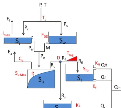
Figure 3. The lumped model structure FLEXL.

also based on our knowledge of the large catchment area and elevation differences.

4.1.1 Snow and interception routine

Precipitation can be stored in snow or interception reservoirs before the water enters the unsaturated reservoir. Basically, the snow routine plays an important role in winter and spring while interception becomes more important in summer and autumn. Here it is assumed that interception happens dur-ing rainfall events when the daily air temperature is above the threshold temperature (Tt; the units of the parameters are listed in Tables 5 and 6) and there is no snow cover, i.e. typ-ically in summer. When the average daily temperature is be-lowTt, precipitation is stored as snow cover, which normally occurs in winter. When there is snow cover and the temper-ature is aboveTt, the effective precipitation (Pe; hereinafter the unit of fluxes is mm d−1) is equal to the sum of rain-fall (P) and snowmelt (M), conditions normally prevailing in early spring and early autumn. Note that snowmelt water is conceptualized to directly infiltrate into the soil, thus ef-fectively bypassing the interception store. In other words, in-terception and snowmelt never happen simultaneously. Their respective activation is controlled by air temperature, precip-itation and the presence of snow cover.

The snow routine was designed as a simple degree-day model as successfully applied in many conceptual mod-els (Seibert, 1997; Uhlenbrook et al., 2004; Kavetski and Kuczera, 2007; Hrachowitz et al., 2013a; Gao et al., 2012). As shown in Eqs. (4) and (5), M is the snowmelt,Sw (the unit of storage is mm) is the storage of snow reservoir, dt(d) is the discretized time step andFDDis the degree day factor, which defines the melted water per day per Celsius degree aboveTt.

The interception evaporation Ei was calculated by po-tential evaporation (Ep) and the storage of interception

reservoir (Si), with a daily maximum storage capacity (Imax) (Eqs. 6, 7, 8).

4.1.2 Soil routine

The soil routine, which is the core of hydrological models used in this study, determines the amount of runoff gener-ation. In this study, we applied the widely used beta func-tion of the Xinanjiang model (Zhao, 1992) to compute the runoff coefficient for each time step as a function of the rel-ative soil moisture. In Eq. (11),Cr(−) indicates the runoff coefficient,Suis the soil moisture content,SuMaxis the max-imum soil moisture capacity in the root zone andβ is the parameter describing the spatial process heterogeneity in the study catchment. In Eq. (12),Peindicates the effective rain-fall and snowmelt into the soil routine; Ru represents the generated flow during rainfall events. In Eq. (13),Rf indi-cates the flow into the fast-response routine;Dis a splitter to separate recharge from preferential flow. In Eq. (14),Rs indicates the flow into the groundwater reservoir. In Eq. (10)

Su,SuMax and potential evaporation (Ep) were used to de-termine actual evaporationEa;Ce indicates the fraction of

SuMaxabove which the actual evaporation is equal to poten-tial evaporation, here set to 0.5 as previously suggested by Savenije (1997); otherwiseEa is constrained by the water available inSu.

4.1.3 Response routine

Equations (15) and (16) were used to describe the lag time between storm and peak flow.Rf(t−i+1)is the generated fast runoff in the unsaturated zone at timet−i+1,Tlagis a parameter which represents the time lag between storm and fast runoff generation,c(i)is the weight of the flow ini−1 days before andRfl(t )is the discharge into the fast-response reservoir after convolution.

The linear-response reservoirs, representing a linear rela-tionship between storage and release, are applied to concep-tualize the discharge from the surface runoff reservoir, fast-response reservoirs and slow-fast-response reservoirs. In Eq. (18),

Qffis the surface runoff, with timescaleKff, active when the storage of the fast-response reservoir exceeds the threshold

Sftr. In Eqs. (19) and (21),QfandQsrepresent the fast and slow runoff;SfandSsrepresent the storage state of the fast and the groundwater reservoirs;KfandKsare the timescales of the fast and slow runoff, respectively, whileQmis the total modelled runoff from the three individual components. 4.2 Model with semi-distributed forcing data (FLEXD) In order to test the influence of model complexity on model performance and model transferability, another benchmark model (FLEXD) based on FLEXLwas developed. The four parallel model structures of FLEXDare identical to FLEXL, but they are run with independent parameter sets (Fig. 4) and semi-distributed input data (see Sect. 3.2), resulting in

1902 H. Gao et al.: Testing the realism of a topography-driven model (FLEX-Topo) – Upper Heihe, China distributed accounting of the four Thiessen polygons and the

seven elevation bands in the study area (Fig. 4). In total, there are 48 parameters for these four Thiessen polygons.

4.3 Topography-driven, semi-distributed models (FLEXT0and FLEXT)

Based on the perceptual model of the Upper Heihe (see Sec-tion “The landscapes and the perceptual model of the Up-per Heihe”), the hypotheses that different observable land-scape units are associated with different dominant hydrolog-ical processes was tested by incorporating these units into hydrological models.

4.3.1 Landscape classification

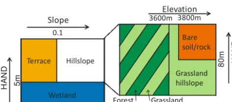
In this study, HAND (Rennó et al., 2008; Nobre et al., 2011; Gharari et al., 2011), elevation, slope and aspect (Fig. 5) were used for deriving a hydrologically meaningful land-scape classification. The stream initiation threshold for es-timating HAND was set to 20 cells (0.16 km2), which was selected to maintain a close correspondence between the de-rived stream network and that of the topographic map. The HAND threshold value for distinction between wetland and other landscapes was set at 5 m, similar to what was used in earlier studies (Gharari et al., 2011). If HAND is larger than 5 m, but the local slope is less than 0.1, the landscape element defines terrace as a landscape unit that connects hillslopes with wetlands. The most dominant landscape in the Upper Heihe, however, is the hillslope, which has been further sep-arated into three subclasses according to HAND, absolute elevation, aspect and vegetation cover (Fig. 5). Thus, hill-slopes above 3800 m and with HAND>80 m, typically char-acterized by bare soil/rock, have been accordingly defined as bare-soil/rock hillslopes. At elevations between 3200 and 3600 m and aspect between 225 and 135◦, or at elevations be-low 3200 m and aspect between 270 and 90◦, hillslopes in the Upper Heihe are generally forested (Jin et al., 2008) and thus have been defined as forest hillslopes. The remaining hill-slopes were defined as grassland hillhill-slopes. From the classi-fication map (Fig. 6b), it can be seen that the landscape clas-sification is similar to the independently obtained land cover map (Fig. 6a) except for the area of wetland, due to different definitions between the land cover map and our classification. Note that wetland and terrace landscape classes have been combined (Fig. 6b), because the area proportion of wetlands varies over time, while terraces may be flooded at times, which can be described by the VCA concept. This combi-nation is unlikely to reduce realism and makes the model simpler. Consequently, the NDVI map has been averaged in accordance with this classification (Fig. 6c).

4.3.2 FLEXT0and FLEXTmodel structures

Based on the landscape classification and the perceptual models for each landscape, different model structures to

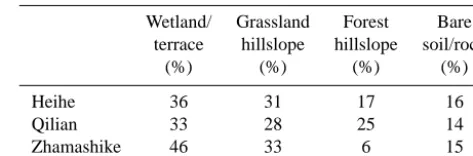
Table 4. Proportion of different landscape units in the study catchments.

Wetland/ Grassland Forest Bare

terrace hillslope hillslope soil/rock

(%) (%) (%) (%)

Heihe 36 31 17 16

Qilian 33 28 25 14

Zhamashike 46 33 6 15

represent the different dominant hydrological processes were assigned to the four individual landscape classes (Table 4). The four model structures ran in parallel, except for the groundwater reservoir (Fig. 7). The snowmelt process was considered in all landscapes using the same method as de-scribed in Sect. 4.1.1.

In the bare-soil/rock class, HOF (RHB), caused by the comparatively low infiltration capacity compared to vegetation-covered soils on hillslopes, is controlled by a threshold parameter (Pt) (Eq. 22). HOF only occurs when the daily effective precipitation (PeB) is larger thanPt:

RHB=max(PeB−Pt,0) . (22)

SOF (RSB), caused by limited storage capacity of the rather shallow soils at high elevations, happens when the amount of water in the unsaturated reservoir exceeds the storage ca-pacity (SuMaxB). Deep percolation from bare soil/rock into groundwater (RpB) is controlled by the relative soil moisture (SuB/SuMaxB) and maximum percolation (PercB):

RpB=PercB

SuB

SuMaxB

. (23)

The actual evaporation (EaB) is estimated by potential evap-oration (EpB) and relative soil moisture (SuB/SuMaxB), which is the same as the calculation of RpB by PercB and SuB/SuMaxB in Eq. (23). The generated surface runoff on the bare soil/rock is separated into the water re-infiltrating (RrB) while flowing on the higher permeable debris slopes and the water directly routed to the channel (RffB) by a sep-arator (DB). As in FLEXD, the lag times are characterized by different lengths in the individual components. The re-sponse process of the surface runoff is controlled by a linear reservoir.

H. Gao et al.: Testing the realism of a topography-driven model (FLEX-Topo) – Upper Heihe, China 1903

29

1

Fig. 4. The semi-distributed model structure FLEX

_{, consisting of four parallel components,}

2

representing one Thiesson polygon each. Each of the parallel components is characterized by

3

an individual parameters set

4

5

6

Fig. 5. Summary of the landscapes classification criteria. The numbers (5m, 80m, 3600m, and

7

0.1)are the criteria for different landscape classes, e.g. <5m for wetland and >5m for terrace

8

and hillslope.

9

10

11

12

Fig. 6. Comparison of land cover(a) and landscape classification maps (b,c), and the NDVI in

13

each land cover (c)

14

15

Slope

Elevation

H A N D H A N D 5m 80 m Grassland hillslope Grassland hillslope Forest hillslope

Figure 4. The semi-distributed model structure FLEXD, consisting of four parallel components, representing one Thiessen polygon each. Each of the parallel components is characterized by an individual parameters set.

29 1

Fig. 4. The semi-distributed model structure FLEXD_{, consisting of four parallel components,} 2

representing one Thiesson polygon each. Each of the parallel components is characterized by

3

an individual parameters set

4

5

6

Fig. 5. Summary of the landscapes classification criteria. The numbers (5m, 80m, 3600m, and

7

0.1)are the criteria for different landscape classes, e.g. <5m for wetland and >5m for terrace

8 and hillslope. 9 10 11 12

Fig. 6. Comparison of land cover(a) and landscape classification maps (b,c), and the NDVI in

13

each land cover (c)

14 15 Terrace Hillslope Wetland Slope 0.1 _Bare soil/rock

3600m 3800mElevation

H A N D H A N D 5m 80 m Grassland hillslope Grassland hillslope Forest hillslope

Figure 5. Summary of the landscapes classification criteria. The numbers (5 m, 80 m, 3600 m and 0.1) are the criteria for different landscape classes, e.g.<5 m for wetland and>5 m for terrace and hillslope.

(QrW) is conceptualized as the dominant hydrological pro-cess due to the shallow groundwater and resulting limited storage capacity. Additionally capillary rise (CR) is repre-sented by a parameter (CRmax) indicating a constant amount of capillary rise. The calculation method of effective rain-fall and actual transpiration is the same as for grassland and forest hillslopes. The lag time of storm runoff in wetland is neglected due to the, on average, comparatively close dis-tance of wetlands/terraces to the channel. The groundwater (Qs) was assumed to be generated from one single aquifer in the catchment and represented by a lumped linear reservoir. In total FLEXTrequires 25 parameters. The final simulated runoff is equal to the sum of runoffs from all landscape ele-ments according to their areal proportions (Fig. 7).

4.4 Model calibration 4.4.1 Objective functions

To allow for the model to adequately reproduce different as-pects of the hydrological response, i.e. high flow, low flow and the flow duration curve, and thereby increase model re-alism, a multi-objective calibration strategy was adopted in

this study, using the Nash–Sutcliffe efficiency (NSE) (Nash and Sutcliffe, 1970) of the hydrographs (INS) to evaluate the model performance during high flow, the NSE of the flow du-ration curve (INSF) to evaluate the simulated flow frequency and the NSE of the logarithmic flow (INSL) which empha-sizes the lower part of the hydrograph.

4.4.2 Calibration method

The groundwater recession parameter (Ks) is not treated as a free calibration parameter but it was rather obtained directly from the observed hydrograph using a master recession curve approach (MRC) (Fenicia et al., 2006). Therefore, Ks was fixed at 90 (d) to avoid its interference with other processes. Together with fixing Ce this results in 10, 40 and 23 free calibration parameters for FLEXL, FLEXD and FLEXT0/T, respectively.

The MOSCEM-UA (Multi-Objective Shuffled Complex Evolution Metropolis-University of Arizona) algorithm (Vrugt et al., 2003) was used as the calibration algorithm to find the Pareto-optimal fronts of the three objective func-tions. There are three parameters to be set for MOSCEM-UA: the maximum number of iterations, the number of com-plexes and the number of random samples that is used to initialize each complex. For the FLEXLmodel the number of iterations was set to 50 000, the number of complexes to 10 and the number of random samples to 1000. To account for increase model complexity, these MOSCEM-UA param-eters of the FLEXDwere set to 50 000, 40 and 3200; those of FLEXTto 50 000, 23 and 2300. The uniform prior parameter distributions of FLEXLand FLEXDare listed in Table 5 and the ones of FLEXT0and FLEXTare given in Table 6. 4.4.3 Constraints on parameters and fluxes in FLEXT Guided by our perceptual understanding of the study catch-ment in the Section on “The landscapes and the perceptual model of the Upper Heihe” and the NDVI map (Fig. 6c), a set of realism constraints for model parameters and simulated

1904 H. Gao et al.: Testing the realism of a topography-driven model (FLEX-Topo) – Upper Heihe, China

29

1

Fig. 4. The semi-distributed model structure FLEX

, consisting of four parallel components,

2

representing one Thiesson polygon each. Each of the parallel components is characterized by

3

an individual parameters set

4

5

6

Fig. 5. Summary of the landscapes classification criteria. The numbers (5m, 80m, 3600m, and

7

0.1)are the criteria for different landscape classes, e.g. <5m for wetland and >5m for terrace

8

and hillslope.

9

10

11

12

Fig. 6. Comparison of land cover(a) and landscape classification maps (b,c), and the NDVI in

13

each land cover (c)

14

15

Terrace Hillslope

Wetland

Slope

0.1 _Bare

soil/rock 3600m 3800m

Elevation

H

A

N

D H

A

N

D

5m

80

m

Grassland hillslope

Grassland hillslope Forest

hillslope

Figure 6. Comparison of land cover (a), landscape classification maps (b, c) and the NDVI in each land cover (c).

Figure 7. Perceptual model and parallel model structures of FLEXTfor the Upper Heihe.

Table 5. Uniform prior parameter distributions of the FLEXLand FLEXDmodels.

Parameter Range Parameters Range

FDD(mm/(d◦C−1)) (1, 8) Ks(d) 90

Tt(◦C) (−2.5, 2.5) Sftr(mm) (10, 200)

Imax(mm d−1) (0.1, 5) Kff(d) (1, 5)

SuMax(mm) (50, 1000) Kf(d) (1, 20)

β(−) (0.1, 5) Tlag(d) (0, 5)

D(−) (0, 1) Ce(−) 0.5

fluxes was developed, similar to what was recently sug-gested by Gharari et al. (2013a). Parameter sets and model simulations that do not respect these constraints were re-garded as non-behavioural parameters and rejected during calibration. The motivation is that by reducing unrealistic pa-rameter combinations, the predictive uncertainty of a model may reduce, although the performance during calibration may be slightly decreased. More specifically, the parame-ters related to interception evaporation and transpiration were

H. Gao et al.: Testing the realism of a topography-driven model (FLEX-Topo) – Upper Heihe, China 1905

Table 6. Uniform prior parameter distributions of the FLEXT0and FLEXTmodel.

Parameters Range Parameters Range Parameter Range Parameter Range Parameter Range

in all 3 for bare for forest for grass for wetland

models soil/rock hillslope hillslope

F_DD (1, 8) S_uMaxB (5, 500) I_maxFH (1, 10) I_maxGH (0, 10) I_maxW (0.1, 10)

(mm/(d◦C−1)) (mm) (mm d−1) (mm d−1) (mm d−1)

Tt (−2.5, 2.5) PmaxB (0.1, 10) SuMaxFH (100, 1000) SuMaxGH (50, 1000) SuMaxW (5, 1000)

(◦C) (mm d−1) (mm) (mm) (mm)

Pt (5, 35) DB (0, 1) βFH (0.1, 5) βGH (0.1, 5) βW (0.1, 5)

(mm d−1) (−) (−) (−) (−)

K_f (1, 20) K_ff (2, 50) C_Rmax (0.01, 2)

(d) (d) (mm d−1)

Ks 90 Kr (1, 9)

(d) (d)

D (0, 1)

(−)

T_lagT (0, 5)

(d)

TlagY (0, 5)

(d)

T_lagQ (0, 5)

(d)

Table 7. The soft data to constrain the automatic calibration.

Soft parameter constraint based on Soft performance constraint perceptual realism based on NDVI map

I_maxFH> I_maxGH E_iFH+E_aFH> E_iGH+E_aGH

ImaxFH> ImaxW EiW+EaW> EiGH+EaGH

SuMaxFH> SuMaxGH> SuMaxW EiGH+EaGH> EaB

S_uMaxFH> S_uMaxGH> S_uMaxB E_aFH> E_aGH Ks> Kf> Kff

Ks> Kf> Kr

Similarly, the annual average evaporative fluxes from wet-land/terrace (EiW+EaW) are assumed to be higher than from the grassland as the latter are more moisture constrained. The evaporative water loss from the bare-soil/rock class (EaB) is the lowest, due to its sparse vegetation cover, limited near-surface storage and lowest temperatures. Furthermore, tran-spiration in forest (EaFH) should be expected to be higher than in grassland (EaGH) because more water is used for biomass production and deeper roots allow access to a larger pool of water.

4.5 Model evaluation

Model evaluation is usually limited to calibration followed by sample validation (Klemeš, 1986). Frequently, split-sample validation can result in satisfactory model perfor-mance as the model is trained by data from the same lo-cation in the preceding calibration period. On the basis of

successful split-sample validation, models and their parame-terizations are then often considered acceptable for predict-ing the rainfall-runoff response at the given study site. It has in the past, however, been observed that many models with adequate split-sample performance failed to reproduce hydrographs even in the nested sub-basins of the calibrated basin (e.g. Pokhrel and Gupta, 2011). In this study, we there-fore applied the calibrated models of different complexity and degrees of input data distribution together with their cal-ibrated parameter sets to two nested catchments to test the models’ transferability and thus the ability to reproduce the hydrological response in catchments they have not explic-itly been trained for. This kind of nested sub-catchment val-idation can, even if it is not an entirely independent valida-tion in the sense of a proxy-basin test (Klemeš, 1986), give crucial information on the process realism and the related predictive power of a model. In this study the hydrological data at the main outfall Yingluoxia (1959–1968) were used for model calibration. Subsequently the model was tested by a split-sample test at the main outfall (1969–1978) and its two nested stations: Qilian (1967–1978) and Zhamashike (1959–1978).

5 Results

5.1 Results of FLEXLand FLEXD

Table 8, as well as Figs. 8a and 9a, illustrate that FLEXL performed quite well in the calibration period with respect

1906 H. Gao et al.: Testing the realism of a topography-driven model (FLEX-Topo) – Upper Heihe, China

Table 8. The averaged results of all the points on the Pareto front of three objective functions of the three models FLEXL, FLEXD, FLEXT0 and FLEXTin calibration, split-sample and nested sub-catchments validation.

Calibration Split-sample Zhamashike Qilian

validation validation validation

INS INSF INSL INS INSF INSL INS INSF INSL INS INSF INSL

FLEXL 0.82 0.99 0.87 0.79 0.95 0.78 0.54 0.79 0.56 0.56 0.87 0.59

FLEXD 0.81 0.99 0.84 0.80 0.96 0.83 0.56 0.82 0.60 0.38 0.67 0.44

FLEXT0 0.82 0.99 0.88 0.80 0.97 0.84 0.60 0.89 0.70 0.68 0.90 0.71

FLEXT 0.80 0.98 0.84 0.78 0.95 0.82 0.65 0.92 0.74 0.71 0.96 0.75

0 0.2 0.4 0.6 0.8 1 10−2

10−1 100 101

Fraction of flow equaled or exceeded [−]

Runoff depth [mm/d]

Calibration FDC of Yingluoxia Observed runoff FLEXL FLEXD FLEXT 0 FLEXT

0 0.2 0.4 0.6 0.8 1 10−2

10−1 100 101

Runoff depth [mm/d]

Validation FDC of Yingluoxia

0 0.2 0.4 0.6 0.8 1 10−2

10−1 100 101

Runoff depth [mm/d]

Validation FDC of Zhamashike

0 0.2 0.4 0.6 0.8 1 10−2

10−1 100 101

Runoff depth [mm/d]

Validation FDC of Qilian

a)

d)

c)

b)

Fraction of flow equaled or exceeded [− Fraction of flow equaled or exceeded [−

Fraction of flow equaled or exceeded [−

] ]

]

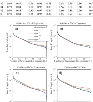
Figure 8. Calibration (a) and validation results for the flow duration curve of four models (FLEXL(lumped model), FLEXD(semi-distributed model with different parameter sets for different Thiessen polygons), FLEXT0(FLEX-Topo model without constraints) and FLEXT (FLEX-Topo model with constraints)) for the entire Upper Heihe (b) and the two tested sub-catchments (c, d). The curves make use of the average value of the parameter sets on the Pareto-optimal front.

to both the hydrograph and the flow duration curve (FDC). In spite of a somewhat reduced performance, the lumped model was also able to reproduce the major features of the catchment response in the split-sample validation (Table 8, Figs. 8b and 9b). Testing the model’s potential in an un-calibrated part of the catchment as if the unun-calibrated parts were ungauged basins (Sivapalan et al., 2003; Hrachowitz et al., 2013b), the performance of FLEXLwas far from sat-isfactory (Table 8, Figs. 8c and d, 9c and d). The valida-tion hydrographs in two tested sub-catchments, which are in the same period as the split-sample validation, are shown in Fig. 9c and d. One interesting observation is that the large

precipitation event at the end of the warm season in 1970 did not generate a flood peak in all three catchments, a char-acteristic that cannot be adequately reproduced by FLEXL (Fig. 9b–d). Similarly, the sub-catchment FDCs (Fig. 8b–d) indicate that FLEXL, while in general mimicking the FDC of the entire catchment well, poorly represents the low flow characteristics of the two sub-catchments.

H. Gao et al.: Testing the realism of a topography-driven model (FLEX-Topo) – Upper Heihe, China 1907

−20 0 20 40

0 3

runoff depth [mm

d

−1]

0 3

−20 0 20 40

0 3

0 3

0 3

15−Apr−670 17−Jul−67 18−Oct−67

3

15−Apr−700 17−Jul−70 18−Oct−70

3

15−Apr−700 24−Jul−70 18−Oct−70

3 0 3

15−Apr−700 17−Jul−70 18−Oct−70

3 0 3 0

3 0 3 −20 0 20 40

0 3 0 3 −20 0 20 40 0 3 Precipitation (mm/d)

Temperature (oC)

Simulated runoff

Observed runoff

a) b)

c)

Zhamashike calibration

Upper Heihe validation

Qilian validation Upper Heihe calibration

FLEXL

FLEXT

FLEXT0

d)

FLEXD

Figure 9. Comparison between observed values (black line) and the envelope of all modelled Pareto-optimal hydrographs (grey shaded area) of four models – FLEXL(lumped model), FLEXD(semi-distributed model with different parameter sets for different Thiessen polygons), FLEXT0(FLEX-Topo model without constraints) and FLEXT (FLEX-Topo model with constraints) – in the calibration period (a), split-sample validation (b) and sub-catchments validation (c, d). Precipitation (blue bars) and temperature (red line) are also shown. The dashed box indicates the September 1970 storm event.

and 9a), the objective functions indicate a slightly poorer calibration performance (Table 8), in spite of two addi-tional parameters in each parallel model component account-ing for differences in channel routaccount-ing lag times. In this study, the reason is potentially related to the uncertainty in the precipitation–elevation relationship and the inappropriate soil moisture distribution dictated by the Thiessen polygons. In the split-sample and Qilian sub-catchment validation (Ta-ble 8, Fig. 8b and d), FLEXDdoes not add value to the re-sults of the lumped FLEXL model which is mostly related to the adverse effects of increased equifinality. However, the validation results in Zhamashike improve with FLEXD, with increased NSE values for both FDC and the hydrograph (Table 8), although base flow is still not reproduced well (Fig. 8c). This indicates that at least for the Zhamashike sub-catchment the distributed precipitation is more representa-tive than catchment-averaged precipitation or that the results

are more sensitive to the heterogeneity of precipitation and temperature input than in the Qilian sub-catchment. In ad-dition, hydrograph inspection revealed that the mismatch of observed and modelled runoff, generated by the large pre-cipitation event at the end of the warm season, was not cap-tured well by the FLEXD either (Fig. 9b–d), although there was a slight improvement (see the reasons in Sect. 6.1). The results of FLEXD indicate that increased model complexity alone, without deeper consideration of the underlying pro-cesses, does not result in a better model transferability. 5.2 Results of FLEXT0and FLEXT

From Table 8 and Figs. 8 and 9, it can be seen that the FLEXT0set-up (i.e. no constraints) results in a similar perfor-mance to FLEXLand FLEXD in calibration and validation, but outperforms the latter two when tested in the two sub-catchments. After adding the constraints, we found that the

1908 H. Gao et al.: Testing the realism of a topography-driven model (FLEX-Topo) – Upper Heihe, China

Table 9. The simulated results of FLEXT.

Bare soil/rock (18 %) Forest hillslope (17 %) Grassland hillslope (31 %) Wetland/terrace (36 %)

P (mm a−1) 481 P (mm a−1) 431 P (mm a−1) 431 P (mm a−1) 410

EaB(mm a−1) 174 EiFH(mm a−1) 125 EiGH(mm a−1) 58 EiW(mm a−1) 87

RpB(mm a−1) 115 EaFH(mm a−1) 257 EaGH(mm a−1) 205 EaW(mm a−1) 220

RrB(mm a−1) 107 RsFH(mm a−1) 15 RsGH(mm a−1) 63 CR(mm a−1) 21

QffB(mm a−1) 77 QfFH(mm a−1) 26 QfGH(mm a−1) 101 QrW(mm a−1) 122

performance of FLEXTin calibration and split-sample vali-dation, as expected (because of the reduced degrees of free-dom) and as indicated by the objective functions (Table 8), is slightly lower than the performance of other models. How-ever, in sub-catchment validation, the performance of FLEXT is significantly better than the other models. This indicates that both the model structure and the constraints on parame-ters and fluxes in FLEXT_{improve model transferability.}

In Table 9, the fluxes modelled by FLEXT, which are the average values of all the results obtained by the pa-rameter sets on the Pareto-optimal fronts, of each landscape class for the entire catchment are given. The water balances of the individual landscape units illustrate clearly the dis-tinct dominant hydrological functions of these individual units as a priori defined by the modeller’s perception of the system. Specifically, the precipitation on bare soil/rock is 481 mm a−1 (18 % proportion of the entire catchment pre-cipitation), 174 mm a−1 (6 %) evaporates and 115 mm a−1 (4 %) infiltrates into cracks and eventually percolates to the groundwater. Overland flow produces 74 mm a−1(3 %), while 112 mm a−1 (4 %) is generated as subsurface flow on shallow soil. A total of 107 mm a−1 (4 %) of the lo-cally generated overland flows re-infiltrates into groundwa-ter (107 mm a−1 (4 %)) due to the high permeability of de-bris slopes at the foot of the mountains while the remain-ing water (77 mm a−1(3 %)) is routed to the stream network with considerable sediment loads. Precipitation on the for-est hillslopes is 431 mm a−1 (17 %), 125 mm a−1 (5 %) of which is intercepted by and evaporates from canopy and for-est floor; 257 mm a−1 (10 %) is modelled as transpiration, while only 26 mm a−1(1 %) and 15 mm a−1(0.6 %), respec-tively, contribute to fast runoff and groundwater recharge, highlighting the dominant evaporation function of this land-scape class. The precipitation on the grassland hillslopes is 431 mm a (31 %), of which 58 mm a−1 (4 %) is intercepted, 205 mm a−1 (15 %) is transpired, 101 mm a−1 (7 %) gener-ates fast runoff and 63 mm a−1 (5 %) recharges the ground-water. For the wetland/terrace, precipitation is 410 mm a−1 (34 %) and in addition around 21 mm a−1 (1.7 %) is con-tributed from groundwater as capillary rise. 87 mm a−1(7 %) is intercepted; 220 mm a−1 (19 %) is consumed by tran-spiration and 122 mm a−1 (10 %) contributes to the fast runoff. These results underline the importance of wet-lands and terraces for peak flow generation. Finally, the

groundwater discharge is 51 mm a−1(12 %), which accounts for 37 % of the total runoff. In total, the modelled runoff depth is 143 mm a−1, which is close to the observed runoff (141 mm a−1). For the simulated total evaporation, it is in-teresting to find that the ratio between forest and wetland is 1.24, which is close to their NDVI ratio (1.27). Simi-larly, the ratio between water loss to atmosphere in wetland and grassland is 1.21, which is also close to their NDVI ra-tio (1.20). These results support the hypothesis that allowing for hydrologically meaningful process heterogeneity in mod-els while imposing realism constraints can produce flux dy-namics that are adequate reflections of reality, increasing our confidence that these models give “the right answers for the right reasons” (Kirchner, 2006).

H. Gao et al.: Testing the realism of a topography-driven model (FLEX-Topo) – Upper Heihe, China 1909

0 20 40

Apr−670 Jul−67 Oct−67

1 2 3 4 5

runoff depth [mm d

−1

]

0 20 40

Apr−700 Jul−70 Oct−70

1 2 3 4

runoff depth [mm d

−1

]

Bare rock/soil Forest Hillslope Grassland Hillslope Wetland/Terrace Groundwater Observed runoff

0 20 40

Apr−700 Jul−70 Oct−70

1 2 3 4

runoff depth [mm d

−1

]

0 20 40

Apr−700 Jul−70 Oct−70

1 2 3 4

runoff depth [mm d

−1

]

Precipitation (mm/d)

Temperature (oC) a) b)

c) d)

Qilian validation Upper Heihe validation Upper Heihe calibration

Zhamashike validation

Figure 10. The hydrograph components of the calibration (a), split-sample validation (b) and sub-catchments validation (c, d), of the FLEXT model (using the average value of the parameter sets on the Pareto-optimal front).

seen that the response to storm events is generally dominated by the flows generated in wetlands/terraces. Connectivity of hillslopes and bare-soil/rock landscapes however, is typically established with some delay and the magnitude of their con-tributions to stream flow, in particular during relatively dry periods, are significantly lower than that of wetlands/terraces (Fig. 10a). This is well illustrated for the September 1970 event shown in the dashed box in Fig. 10b–d: while to some degree all the landscapes eventually contributed to the runoff, the wetland/terrace responded directly to the storm whereas the limited response of hillslopes and bare soil/rock con-tributed to the peak flow later.

6 Discussion

6.1 Why did FLEXTperform better than FLEXLand FLEXD?

Some clarification can be achieved by comparing the ob-served precipitation duration curves (PDC) and FDCs. From Fig. 11a it can be concluded that the entire Upper Heihe re-ceives the lowest catchment-average precipitation input both in the original forcing data and the elevation-corrected pre-cipitation, while being characterized by the largest runoff yield (Fig. 11b). The Qilian sub-catchment, in contrast, re-ceives the largest amount of precipitation, but with lower runoff yield. The Zhamashike sub-catchment is characterized

by similar precipitation input as the entire Upper Heihe, but exhibits much higher peak flows and lower base flows than both the entire catchment and the Qilian sub-catchment. These distinct catchment hydrological functions are difficult to reconcile in one lumped model, representing a specific rainfall-runoff relationship. Moving to a different catchment or maybe only even to a sub-catchment is likely to change the relative proportions of landscapes, thus leading to a misrep-resentation of the lumped process heterogeneity and thus re-duced model performance in the new catchment. A semidis-tributed approach like FLEXT, in contrast to FLEXL and FLEXD, offers more flexibility in adapting the model to the ensemble of processes in a more realistic way other than the lumped ones trained by adjusting it to the hydrograph, which most likely oversimplifies the catchment heterogeneity. This underlines the increased importance and benefit of more de-tailed, yet flexible expert-knowledge-guided process repre-sentations compared to focusing on mere parameter calibra-tion of lumped models.

The potential reason for overestimating the runoff in the Zhamashike sub-catchment for FLEXLand FLEXD(Fig. 8c) is that these two models do not adequately represent the increased importance of evaporation from wetland/terrace. Similarly, the reason for overestimating flow in the Qilian sub-catchment (Fig. 8d) is that these two models cannot ac-commodate the increased evaporation of forests as much of the Upper Heihe, for which the models were calibrated, is

1910 H. Gao et al.: Testing the realism of a topography-driven model (FLEX-Topo) – Upper Heihe, China

33 1

Fig. 11. The comparison of three observed precipitation duration curves (a) and flow 2

duration curves (b) 3

4

-0.020 0 0.02 0.04 0.06 0.08 0.1 1

2 3 4 5 6

Fraction of flow equaled or exceeded [-]

Runof

f dept

h [

m

m

/d]

Upper Heihe River Basin Qilian

Zhamashike

-0.020 0 0.02 0.04 0.06 0.08 0.1 5

10 15 20 25 30 35 40 45

Fraction of precipitation equaled or exceeded [-]

Pr

ec

ipi

tat

ion [

m

m

/d]

Upper Heihe River Basin Qilian

Zhamashike

Upper Heihe corrected by elevation Qilian corrected by elevation Zhamashike corrected by elevation

b) a)

Figure 11. The comparison of three observed precipitation duration curves (a) and flow duration curves (b).

covered by grassland hillslope and bare soil/rock, character-ized by lower evaporation rates than the other landscapes. On the other hand, both FLEXL and FLEXD overestimate the baseflow (Fig. 8c and d). This can potentially be linked to neglecting capillary rise in the wetland/terrace, which in-fluences both the baseflow and the evaporation of this land-scape element. When capillary rise in FLEXTis considered, the groundwater feeds the unsaturated reservoir in the wet-land, which not only reduces the base flow but also increases the amount of water available for transpiration and eventually evaporation. This hydrological process is especially impor-tant in the Zhamashike sub-basin, where higher peak flows and lower base flow happen simultaneously.

The results support the potential of FLEXT and its pa-rameterization to be spatially and scalewise better transfer-able than lumped model structures, such as FLEXLor semi-distributed models such as FLEXD, which do not explicitly allow for changing proportions of landscape units with dis-tinct hydrological function (see Sect. 5.2). In summary, the FLEXT model set-up, informed by topography, divided the catchments into four topographic subunits, representing dif-ferent dominant hydrological process ensembles. This kind of modelling strategy allowed enough flexibility to capture the different functional behaviours of the three study catch-ments simultaneously (Table 8, Figs. 9–11).

6.1.1 Specific rainfall/snowfall-runoff events

Some modelled events, such as the rainfall/snowfall–runoff event in Fig. 10a, also illustrate that FLEXT is generat-ing internal flow dynamics that better reflect the modeller’s perception of the catchment processes. It can be seen that FLEXT could reproduce the instantaneous response of the wetlands to the storm and the delayed and limited response of other landscapes. As discussed above, another interesting event was observed in September 1970. During that storm the highest daily precipitation of the available record was

observed, while, however, producing only a relatively in-significant runoff peak, both in the Upper Heihe and its sub-catchments (Fig. 9). Both FLEXL and FLEXD failed to ad-equately reproduce this event and modelled a much larger peak flow. Significant precipitation measurement error can be excluded, as the event was observed in similar magni-tudes at all gauges available for this study. The failure of FLEXLand FLEXD to adequately respond to this event can be linked to several reasons. Firstly, the lumped accounting of the snowmelt in FLEXLcan partly be the reason because the lumped model does not consider the change of temper-ature and then the type of precipitation with elevation. The lumped model treats the precipitation as rainfall in the entire catchment when the average daily air temperature is above the rain/snow temperature threshold. However, there could be snowfall in high elevation zones, when the catchment average temperature is slightly above the threshold temper-ature. Likewise, there could be rainfall in lower elevation zones when the catchment average temperature is below the threshold. The temperature record (Fig. 9) clearly shows the low average air temperature on the same day as the large pre-cipitation event. This could partly explain the limited runoff response to this specific storm event, as the modelled results obtained from FLEXDare somewhat closer to the observed response than the results of FLEXL(Fig. 9b and d).

H. Gao et al.: Testing the realism of a topography-driven model (FLEX-Topo) – Upper Heihe, China 1911 the precipitation was in the form of rainfall. The

tempera-ture and precipitation records show that the preceding days were dry and warm (Fig. 10), translating into comparatively elevated evaporation and, linked to that, relatively high soil moisture deficits. In addition, the deep root zone on the forest hillslopes provides considerable storage capacity in the soil before discharge is generated. At a higher elevation, which is mainly characterized by bare soil/rock and grassland hill-slopes, the precipitation was in a solid state, subsequently stored as snowpack. When the temperature increased again in the following days, the snow melted gradually. However, due to the slow melt rates and the dry antecedent conditions, the snowmelt water was almost completely infiltrated into the groundwater and did not contribute to the storm flow, even when the temperature increased several days later (Fig. 10b– d). Therefore, there is apparently enough information, not only in landscapes but also in the observed discharge, to pa-rameterize the FLEXTmodel. In summary, FLEXTallowed the low and high elevation areas to reduce the storm flow for this specific event by different mechanisms, resulting in a very limited response to the event, in close agreement with the observed response.

6.1.2 Realism testing of FLEXTmodel

The FLEXT model is based on landscape classification, which is an observable prior to enhance model realism. Sub-sequently, based on our knowledge and understanding of different dominant hydrological processes in different land-scapes, we assigned suitable hydrological process represen-tations to these landscapes to highlight landscape hetero-geneity. Significant differences in hydrological function, for example between wetland and hillslope, are well documented by a wide range of experimental studies (e.g. McGlynn and McDonnell, 2003; Seibert et al., 2003; Molenat et al., 2008; Jencso et al., 2009; Detty and McGuire, 2010). The consid-eration of landscape heterogeneity, reflected in runoff gener-ation mechanisms and differences in water budgets, makes the FLEXTmodel perform better than FLEXLand FLEXD, reproducing hydrographs (Fig. 9) but also FDCs (Fig. 8), as emergent catchment properties. The suggested model hy-potheses were not only tested for temporal transferability be-tween calibration and validation periods, but also for spa-tial transferability to sub-catchments. This successful trans-ferability (Table 8; Figs. 8 and 9) is strong supporting ev-idence for the hypothesis that landscape carries crucial in-formation on hydrological function and it illustrates that, by allowing for increased process heterogeneity in models, their degree of realism, i.e. their skill to adequately repre-sent critical features in response dynamics, increases. More convincingly, the benchmark model (FLEXD) with a higher number of parameters (40 free parameters) did not improve transferability, even with nearly twice the number of param-eters as in FLEXT(23 free parameters). However, note that here “realism” is not primarily and necessarily linked to an

improved fit of the hydrograph. It is rather linked to the in-corporation of more knowledge available from observation and experiments, thereby allowing the development of mod-els whose internal and external dynamics correspond with this information, which in turn increases model realism.

Note that this paper aims to test the realism of models, meaning that it investigates to which degree a more realistic representation has been achieved, but it does not intend to claim that the developed model is realistic in absolute terms. In that respect it emphasizes that model realism should al-ways be seen in relation to uncertainties arising from data error as well as from the choice of constitutive functions and parameters. In this paper, a detailed analysis of the influence of these uncertainties was omitted as this was beyond the scope of this research. Further, some of the hypotheses of the proposed model structure could not be tested individually for lack of available data. They will be further investigated dur-ing future research, usdur-ing additional information. Thirdly, at this point, the interpretation is only valid in the study catch-ment and subsequent studies will have to test this hypothesis further in other regions in order to evaluate the generality of these findings.

6.2 Translating topography information into hydrological models

It is intriguing to find that the landscape classification based on topography information (HAND, slope, elevation and as-pect) closely reflects the patterns and shapes of the land cover map (Fig. 6a and b). In other words, it clearly illustrates that topography has great influence on the energy and water avail-ability and the evolution of vegetation cover. Certain types of vegetation cover evolve under specific topographic condi-tions. Elevation greatly influences the amount of precipita-tion and available energy. HAND and slope are two impor-tant factors defining water retention and drainage. Aspect in-fluences the energy balance and precipitation. Normally, the south-facing hillslopes receive more solar energy. Thus, the potential evaporation on the south-facing hillslopes is larger than on north-facing ones, while aspect influences the distri-bution of forest and grassland in arid/semi-arid regions.

Topography does not only directly influence the ground-water level and the occurrence of saturation overland flow, but it also controls the soil and vegetation cover in certain ge-ological and climatic condition, and consequently the domi-nant hydrological processes (Savenije, 2010). The presented modelling approach can therefore be seen as a step towards making more efficient use of topographic information for use in conceptual hydrological models. The successfully linked topographic information, land cover classification and hy-drological model structure supports the hypothesis that to-pographic information can be used to distinguish landscape elements with different hydrological functions (Wagener et al., 2007; Savenije, 2010).

1912 H. Gao et al.: Testing the realism of a topography-driven model (FLEX-Topo) – Upper Heihe, China 6.3 The value of soft data in hydrological modelling

(FLEXT0vs. FLEXT)

Hydrological modelling should also be seen as an art (Savenije, 2009). To ensure that models better reflect our understanding of reality we should make use of our experi-ence and creativity. In addition to available data, hydrologists often have extensive, yet sometimes only semi-quantitative expert knowledge about specific study sites. However, this “soft” knowledge is with some exceptions (e.g. .Seibert and McDonnell, 2002, 2013), regularly underexploited in hydro-logical modelling. In general four types of soft data can be valuable for hydrological modelling. The first one is our ex-plicit or inferred knowledge of the hydrological processes occurring in reality. For example, in this study, streams in high elevation tributaries, characterized by a dominance of relatively erodible bare soil/rock, exhibit relatively high lev-els of turbidity (Fig. 2e), thus indicating the importance of soil erosion, which in turn supports the existence of Horto-nian surface runoff in these locations. Another type of “soft” data is the expert knowledge on meaningful acceptable prior parameter ranges, such as the maximum storage of the un-saturated reservoir at the catchment scale (SuMax), which is closely linked to rooting depth and soil structure and strongly depends on the ecosystem. The third kind of valuable “soft” data is the understanding of the relative magnitude of specific parameters in different landscapes (Gharari et al., 2013a), providing further constraints on model parameters, and elim-inating unrealistic parameter combinations. For example, in this study it was argued that forest canopy, undergrowth and litter on forested hillslopes can intercept more precipitation (ImaxFH) than grass-dominated hillslopes (ImaxGH) (Table 7). Fourthly, simulation results can be constrained by “soft” data, such as NDVI maps indicating inequalities between for-est and grassland transpiration (Table 7). Making use of these four types of soft data, a landscape driven model, FLEXT, based on our understanding of the hydrological processes in the Upper Heihe, was developed and constrained. Although the use of these additional constraints resulted in a slightly reduced calibration performance of FLEXTas compared to the FLEXT0set-up, the more successful sub-catchments val-idation illustrated the value of soft data and clearly indicated that the efficient use of soft data allows for a more realistic representation of catchment heterogeneity, leading to higher predictive power.

6.4 The role of forest in the Upper Heihe

Since forest is an important land cover in the Upper Heihe and many other catchments, the hydrological impact of for-est is essential for understanding the catchment water cycle (Andréassian et al., 2004; Lyon et al., 2012), but also for an efficient implementation of water resource management poli-cies. The role of forest on the catchment scale is subject of

ongoing discussion in ecohydrology (Moore and Wondzell, 2005; Sriwongsitanon and Taesombat, 2011).

Various earlier studies found very diverse conclusions (Bosch and Hewlett, 1982; Robinson et al., 1991; Sahin and Hall, 1996; Andréassian, 2004; Moore and Wondzell, 2005). In this study, the FLEXT model generated little runoff in forested hillslopes in the Upper Heihe, with most of the rain-fall on the forest being intercepted and transpired. In ad-dition, these results are supported by other studies in this catchment based on remote sensing information (Tian et al., 2013), statistical analysis (Wang et al., 2011), paired catch-ment analysis in this region (Huang et al., 2003; Qin et al., 2011) and the simulation of an ecohydrological model (Yu et al., 2009). Also, field observations and experimen-tal studies in the Upper Heihe (B. Ye, personal communi-cation, 2012) gave evidence of limited runoff from forests. This phenomenon is most likely linked to the climatic con-ditions in the Upper Heihe. Since the precipitation in this region reaches on average only 430 mm a−1, with a maxi-mum observed daily catchment average precipitation of be-low 45 mm d−1(corrected by elevation), with ample storage available in the root zone, the forest hillslopes in the Upper Heihe remain largely below the moisture content necessary to establish connectivity conditions necessary to significantly contribute to storm flow.

7 Conclusions