Regional analysis of parameter sensitivity for simulation of streamflow and hydrological fingerprints

https://doi.org/10.5194/hess-22-203-2018 © Author(s) 2018. This work is distributed under the Creative Commons Attribution 4.0 License.

Regional analysis of parameter sensitivity for simulation of

streamflow and hydrological fingerprints

Simon Höllering1, Jan Wienhöfer1, Jürgen Ihringer1, Luis Samaniego2, and Erwin Zehe1

1_{Karlsruhe Institute of Technology (KIT), Karlsruhe, Germany} 2_{Helmholtz Centre for Environmental Research, Leipzig, Germany}

Correspondence:Simon Höllering ([email protected]) Received: 20 July 2017 – Discussion started: 21 July 2017

Revised: 13 October 2017 – Accepted: 19 November 2017 – Published: 11 January 2018

Abstract. Diagnostics of hydrological models are pivotal for a better understanding of catchment functioning, and the analysis of dominating model parameters plays a key role for region-specific calibration or parameter transfer. A major challenge in the analysis of parameter sensitivity is the as-sessment of both temporal and spatial differences of parame-ter influences on simulated streamflow response. We present a methodological approach for global sensitivity analysis of hydrological models. The multilevel approach is geared to-wards complementary forms of streamflow response targets, and combines sensitivity analysis directed to hydrological fingerprints, i.e. temporally independent and temporally ag-gregated characteristics of streamflow (INDPAS), with the conventional analysis of the temporal dynamics of parameter sensitivity (TEDPAS).

The approach was tested in 14 mesoscale headwater catch-ments of the Ruhr River in western Germany using simula-tions with the spatially distributed hydrological model mHM. The multilevel analysis with diverse response characteristics allowed us to pinpoint parameter sensitivity patterns much more clearly as compared to using TEDPAS alone. It was not only possible to identify two dominating parameters, for soil moisture dynamics and evapotranspiration, but we could also disentangle the role of these and other parameters with reference to different streamflow characteristics. The combi-nation of TEDPAS and INDPAS further allowed us to de-tect regional differences in parameter sensitivity and in sim-ulated hydrological functioning, despite the rather small dif-ferences in the hydroclimatic and topographic setting of the Ruhr headwaters.

1 Introduction

1.1 Analysis of parameter influences

The role of hydrological model parameters has been studied for a long time. The ill-posed nature of problems in hydro-logical modelling led to the awareness that parameter sets are not uniquely identifiable (Beven, 1993) and to the re-lated branches of uncertainty assessment (e.g. Gupta et al., 1998) and automated parameter estimation (e.g. Hogue et al., 2000). Both are closely related to the sensitivity of model re-sults to parameter variations. While a number of topics are often subsumed under sensitivity analysis, underlying objec-tives and methodological approaches can substantially dif-fer from case to case (van Griensven et al., 2006; Saltelli et al., 2008; Zajac, 2010; Razavi and Gupta, 2015). Local and global strategies of sensitivity analysis have been shown to be helpful at different stages of the modelling process (Mc-Cuen, 1973; Hamby, 1994; Sieber and Uhlenbrook, 2005; Razavi and Gupta, 2015). Analogous to the number of dif-ferent objectives and methods to assess parameter sensitiv-ity, the results are subject to different forms of interpreta-tion (Razavi and Gupta, 2015). The way that the outcome of sensitivity analysis is evaluated and illustrated can strongly affect the conclusions that are drawn. In this regard, results of sensitivity analysis can widely differ if varying objective functions are considered for the evaluation of parameter in-fluences (Demaria et al., 2007; Wagener et al., 2009); for a comprehensive overview see Reusser et al. (2011).

pointed out that parameter sensitivity should be analysed in a time-dependent context, as hydrological systems are sub-ject to temporally dynamic processes. Guse et al. (2016b) argued that the study of temporal variations in sensitivity is essential to learn about the relation between dominant pa-rameters and governing processes under changing hydrologi-cal conditions. The characterisation of temporal dynamics of parameter sensitivity (TEDPAS) has been accomplished in diverse ways (Cloke et al., 2008; Cibin et al., 2010; Reusser et al., 2011; Reusser and Zehe, 2011; Herman et al., 2013; Sanadhya et al., 2013; Guse et al., 2014; Pfannerstill et al., 2015; Pianosi and Wagener, 2016). The choice of the tem-poral resolution is an important factor which clearly influ-ences the way parameters are identified and how inferinflu-ences on related processes are made (Tang et al., 2007; Massmann and Holzmann, 2012; O’Loughlin et al., 2013). Necessarily, the timescale of sensitivity analysis is selected in accordance with the objective of the study and the dynamics of the sys-tem under investigation. The importance of parameters sys- tem-porally varies as short periods of high flow alternate with longer periods of low flow (Massmann et al., 2014).

When model calibration and verification come into play, analysis of parameter sensitivity provides valuable informa-tion on the importance of each input factor in regard to sim-ulated model output. On this basis, it can be decided for each parameter whether its value should be determined exactly, or if it could even be completely excluded, fixed at prede-termined values (Reusser et al., 2011). Preferably, sensitiv-ity analysis minimises the necessary number of parameters as hydrological models are often subject to overparameteri-sation (Beven, 2001; Kirchner, 2006; van Werkhoven et al., 2009; Samaniego et al., 2010b).

A common goal of sensitivity-guided studies dealing with an identification of dominant processes is the achievement of a suitable representation of real-world hydrological pro-cesses by understanding the reasons for model defective-ness. If non-sensitive parameters are detected, an indication of model structural deficits (Kirchner, 2006; Gupta et al., 2012), or a lack of the adequate model response target data might be given. Sensitivity analysis is, not just recently, con-sidered as a helpful diagnostic tool to identify structural and performance deficits of hydrological models (McCuen, 1973; Sieber and Uhlenbrook, 2005; Yilmaz et al., 2008; Kavetski and Clark, 2010; Guse et al., 2014; Pfannerstill et al., 2015). Reusser and Zehe (2011) showed that a combined analysis of the temporally varying parameter dominance (sensitivity analysis) and model performance (error analysis) can effec-tively detect structural inadequacies of model components for a specific landscape.

1.2 Fingerprint-based sensitivity analysis

The characterisation of catchment functioning and the un-derlying hydrological processes can be addressed in various ways, at multiple scales and levels of complexity. Fingerprint

metrics (hereinafter also referred to as fingerprints) are signa-tures of dynamic catchment response that change on different temporal and spatial scales (Sivapalan, 2005; Wagener et al., 2007; Winsemius et al., 2009).

In hydrological modelling, multiple fingerprint metrics have been adopted to enhance model evaluation beyond the minimisation of streamflow residuals. Fingerprints of catch-ment functioning may be classified into measures based on single-value (statistical) streamflow indices, and those based on characteristic curves, e.g. (cumulative) frequency curves, regime curves, or double mass curves. Examples for the two kinds of fingerprint metrics are the runoff ratio and the flow duration curve, respectively. Representatives of both categories can be selected to describe single components of streamflow regimes, namely the magnitude, frequency of oc-currence, duration, timing, and flashiness of flow events (Poff et al., 1997; Olden and Poff, 2003), or of the general hydro-logical variability at different spatial and temporal scales.

In a comprehensive analysis of catchment functioning in order to understand dominant processes, the use of a sin-gle criterion is often not sufficient. Therefore, hydrologi-cal fingerprints have been jointly used as multivariate ob-jectives to estimate the parameters of hydrological models (Shamir et al., 2005a, b; Pokhrel et al., 2008; Castiglioni et al., 2010) or to assess model performance and evaluate model structures (Farmer et al., 2003; Gupta et al., 2008; Yil-maz et al., 2008; Clark et al., 2011; Euser et al., 2013; Vrugt and Sadegh, 2013).

Sensitivity analysis related to streamflow characteristics was formerly mostly applied prior to model evaluation (e.g. Atkinson et al., 2003). For sensitivity analysis, different op-tions have been selected as hydrological target variables. Sensitivity analysis to assess the influence of parameters can be directed to (i) simulated streamflow, (ii) different objective functions (e.g. van Werkhoven et al., 2009; Wagener et al., 2009; Herman et al., 2013; Sanadhya et al., 2013), (iii) simu-lated hydrological processes (e.g. Massmann and Holzmann, 2015; Pfannerstill et al., 2015; Guse et al., 2016a), or (iv) dif-ferent hydrological fingerprints (this study). Previous stud-ies applied fingerprint metrics but based the analysis of pa-rameter sensitivity on only a few aspects of streamflow (e.g. limb densities; Shamir et al., 2005a) or on single (statisti-cal) streamflow indices of different aggregation timescales (Shamir et al., 2005b).

variable streamflow magnitudes of two distinct streamflow regimes.

1.3 Objectives, research questions and approach The main objectives of this study are to analyse the parameter sensitivity of a mesoscale hydrological model for the simula-tion of streamflow response and hydrological fingerprints at a set of headwater catchments of the Ruhr in Germany. The approach extends TEDPAS along two avenues: the first is to investigate TEDPAS results in more detail to derive parame-ter sensitivities in different hydrological conditions; the sec-ond is to direct the analysis to other, temporally independent characteristics of streamflow response (INDPAS).

With this approach we explore the following three research questions:

– Which sensitive parameters can be identified with re-gard to specific hydrological response characteristics? – How does parameter sensitivity change with different

hydrological objectives (response targets) applied in global sensitivity analysis?

– How does parameter sensitivity change among different catchments with slightly distinct physiographic and hy-droclimatic conditions?

The methodological approach combines streamflow hy-drographs and fingerprint metrics as response targets for the analysis of first-order partial parameter sensitivity. The anal-ysis rests on a state-of-the-art distributed hydrological model and is structured in the following steps:

– combining the application of a hydrological model with global sensitivity analysis to generate an ensemble of parameter sets;

– deriving fingerprint metrics (single-value indices and characteristic curves) from simulated streamflow time series;

– analysing parameter sensitivity to temporally resolved dynamics of streamflow response (TEDPAS);

– analysing parameter sensitivity to both temporally ag-gregated (single-value indices) and temporally indepen-dent (characteristic curves) characteristics of stream-flow (INDPAS);

– assessing differences in parameter sensitivity between the two different methodological approaches (TEDPAS and INDPAS), and between the analysed headwaters. In the study we will thus complement sensitivity analysis based on TEDPAS with fingerprint metrics of streamflow re-sponse (INDPAS), which include both temporally aggregated

single-valued indices and temporally independent character-istic curves. In cases where charactercharacter-istic curves (e.g. the FDC) are used, changes in parameter sensitivity will be anal-ysed for changes in the independent variable (e.g. streamflow exceedance probability). We focus the study on the headwa-ters of the Ruhr catchment in western Germany based on available data sets.

From this we expect to pinpoint dominant parameters re-lated to individual process components and to ease the in-terpretation of parameter sensitivity detached from the vari-ability of timescales. Bearing in mind the complexity of the evaluation of spatially and temporally distributed model re-sponses, our multilevel approach aims at providing further insight into the dominance of model parameters and related streamflow response processes.

2 Methods and models

First we detail the fingerprint metrics used to characterise streamflow response (Sect. 2.1). We implemented the Fourier amplitude sensitivity test (FAST; Sect. 2.2) to analyse the mesoscale hydrologic model (mHM, Sect. 2.3) in the Ruhr headwater catchments. Focusing on eight global mHM pa-rameters (Sect. 2.4), we employed two different forms (TEDPAS and INDPAS) of simulated streamflow response (Sect. 2.5) in the sensitivity analysis. Finally, we introduce the catchment of the Ruhr River and the headwaters which were selected for this study (Sect. 2.6.1), and specify the data used for the analysis (Sect. 2.6.2).

2.1 Fingerprint metrics

Fingerprint metrics are often used in hydrology for charac-terising the hydrological response of catchments (Olden and Poff, 2003; Yadav et al., 2007; Yilmaz et al., 2008; Win-semius et al., 2009). The fingerprint metrics used in this study included single-value indices and the flow duration curve as an example for catchment-characteristic curves. These fin-gerprints were derived from model results and precipitation data (see Sect. 2.6.2), respectively.

Table 1.Temporally aggregated single-value fingerprint metrics derived from FAST-mHM simulated streamflow and observed precipitation time series, serving as model response targets for sensitivity analysis (INDPAS).

Response characteristic Fingerprint metric Abbreviation Unit Derivation

Water balance Runoff ratio RR (–) QTotal/ PTotal

Streamflow variability Coefficient of variation CV (–) σ / µ

Frequency of flow events High pulse count HPC (yr−1) (number of time steps

Q >3×Qmean)/ years

Rate of change in streamflow Slope of flow duration SLFDC (%) Slope of FDC between 33 and 66 %

curve Qexceedance

High-flow conditions High flow discharge HFD (–) Q5th percentile/ Qmedian

Low-flow conditions Baseflow index BFI (–) QBaseflow/ QTotal

Streamflow recession Recession time constant RTC (d) Mdn (time required forQto

reach 1/e×Q_Peak)

Streamflow autocorrelation Autocorrelation time ACT (d) Lag time required for AC function

structure to decrease below 0.5

Q: streamflow;P: precipitation;σ: standard deviation; µ: mean; Mdn: median; AC: autocorrelation.

not be directly determined from streamflow hydrographs. In-stead, the FDC was used as a basis for its derivation. The eight single-value fingerprints were implemented as model response targets for sensitivity analysis (Sect. 2.5.2).

As an example for more complex characteristics than single-valued indices, we also used entire flow duration curves as model response targets for sensitivity analysis (Sect. 2.5.2).

2.2 Fourier amplitude sensitivity test (FAST)

FAST is a partial variance-based method to determine first-order sensitivities of parameter changes on the outcome of monotonic and non-monotonic numeric models (Cukier et al., 1973; Schaibly and Shuler, 1973; Cukier et al., 1975). The general idea of FAST is (a) to vary parameters of interest with independent frequencies along a predefined number of model runs, and (b) to perform a Fourier analysis of the simu-lated target variable across the ensemble of model runs to ob-tain a power spectrum. In the case of TEDPAS, the spectrum is calculated for each simulation time step. The varianceσ_i2

that is explained by a parameteriis determined by normalis-ing the correspondnormalis-ing power with the total power in the spec-trum, which corresponds to the total varianceσ_tot2 within the model ensemble. The sensitivity to model output of param-eteriis then calculated as the partial variance, which is the ratioσ_i2/σ_tot2. Parameter interactions, i.e. higher-order sensi-tivity, are not detected by this method. For more details on FAST the reader is referred to Reusser et al. (2011).

FAST was originally applied to study parametric model sensitivities of chemical reaction systems. In recent decades, the method has been used and evaluated in a variety of fields such as hydrogeology (Fontaine et al., 1992), atmospheric sciences (Rodríguez-Camino and Avissar, 1998), geologic nuclear waste disposal modelling (Lu and Mohanty, 2001), food safety risk assessment (Frey and Patil, 2002), or

eco-logic forestry (Song et al., 2013). A number of studies treat the application of FAST in hydrological modelling (Reusser et al., 2011; Reusser and Zehe, 2011; Sanadhya et al., 2013; Guse et al., 2014; Pfannerstill et al., 2015; Guse et al., 2016a, b).

FAST is a highly efficient computational method that re-quires significantly fewer model runs to yield similar results for parameter sensitivity than other approaches (Saltelli and Bolado, 1998; Reusser et al., 2011). The number of model runs (hence parameter sets) in FAST is determined by the number of analysed model parameters. This means that al-ways the same number of model runs is required for a given number of parameters, independent of model, catchment or type of parameter.

2.3 Mesoscale hydrologic model (mHM)

The mHM (Kumar et al., 2010; Samaniego et al., 2010b) accounts for diverse processes of the hydrological cycle: canopy interception, evapotranspiration, snow, soil moisture dynamics, overland flow, infiltration, interflow, subsurface storage, groundwater recharge, baseflow, discharge attenua-tion, as well as flood routing. The mHM is conceptualised on the basis of grid cells, and has been applied to a wide range of mesoscale river catchments (101–104km2; Kumar et al., 2010; Samaniego et al., 2010a, 2011; Cuntz et al., 2015; Rakovec et al., 2016). Gridded information is imple-mented in mHM at three levels: morphology (level 0), hy-drology (level 1), meteorology (level 2), withl0l1 ≤ l2

denoting the relative sizes of the grid cells at the respective data level (Kumar et al., 2010).

1 are derived from physiographic characteristics at level 0 using (pedo-)transfer functions with coefficients (in the fol-lowing referred to as global mHM parameters). Hence, mHM is calibrated indirectly, by altering the 52 level-0 parameters of the transfer functions instead of the hydrological level-1 parameters. This procedure not only reduces the problem of overparameterisation and the dependence on specific hy-drological scales (Beven, 2001) but also reduces the amount of time that is needed for grid-wise calibration (Samaniego et al., 2010b).

2.4 Model setup for sensitivity analysis

To facilitate the selection of the most sensitive parameters, we first carried out a preliminary FAST analysis at the lo-cal slo-cale for gauge Wenholthausen (WEN; Fig. 1) includ-ing all 52 global mHM parameters to reveal parameter sen-sitivities to streamflow simulations. For this initial analysis, 21 803 model runs were conducted and the streamflow hy-drographs were analysed with FAST. We found 14 parame-ters with a maximal sensitivity value of more than 0.01 (1 %). When inspecting the model equations we identified correla-tions between these parameters, which led to the removal of six parameters from this set.

The eight uncorrelated parameters (Table 2) were used for the regional sensitivity analysis in the 14 headwater catch-ments. All other mHM parameters were kept fixed on cali-brated values found via global automatic optimisation using the dynamically dimensioned search algorithm (Tolson and Shoemaker, 2007) at WEN for the period 2002 to 2006. The value ranges for the parameters were selected from mHM lit-erature (Samaniego et al., 2014), partly extended based on the results from the preliminary analysis. For eight param-eters, the FAST method requires 243 model runs based on different parameter combinations originating from variation with independent frequencies inside the parameter ranges (Fig. 2). The same 243 combinations of mHM parameter sets were used for streamflow simulations in each of the 14 catch-ments. Differences between catchments in terms of hydrocli-matic forcing and physiographic attributes were included in the model by the locally specific meteorological and morpho-logical input on data levelsl2andl0.

The hydrological model levell1and the meteorologicall2

of mHM were set to a spatial resolution of 1 km, whereas for level 0 with the physiographic catchment data (morphology), a finer resolution ofl0=200 m was selected as an adequate

spatial discretisation. Model simulations were conducted for each of the 14 headwater catchments (see Sect. 2.6.1) with a daily time step for the 10-year period of 1997 to 2006.

2.5 Sensitivity analysis

We analysed the parameter sensitivity in different forms to be able to evaluate the dominance of parameters and to poten-tially detect local differences among the headwaters related

to various aspects of streamflow response in a more specific way. We used simulated streamflow hydrographs (TEDPAS; Sect. 2.5.1) and both temporally aggregated and temporally independent fingerprint metrics of simulated streamflow re-sponse (INDPAS; Sect. 2.5.2) as model rere-sponse targets for the sensitivity analyses.

2.5.1 TEDPAS – temporal dynamics and sensitivity duration

Using simulated hydrographs with FAST provided daily time series of partial parameter sensitivities for each headwater catchment for the simulation period 1997–2006. These tem-poral dynamics of parameter sensitivity (TEDPAS; Reusser et al., 2011) were analysed and compared for the Ruhr head-water catchments (Sect. 3.1).

We also calculated sensitivity duration curves (SDCs) for each parameter, which we defined in analogy to other well-known cumulative frequency curves like the FDC. Each SDC is specific for one of the eight parameters, for one catch-ment and for the period (1997–2006) in which sensitivity analysis is performed. SDCs were developed for each catch-ment by arranging the daily sensitivity values from FAST by magnitude in ascending order and by plotting them as a line against the percentage of time during which the sensitivity equalled or exceeded the specified values. Sensitivities were normalised by the highest sensitivity value found for each pa-rameter among all headwaters. These curves reveal whether a parameter is consistently (non-)sensitive or if its importance changes during the simulation period (Sect. 3.2).

2.5.2 INDPAS – parameter sensitivity to fingerprint metrics

For each catchment we calculated eight single-valued finger-print metrics (Sect. 2.1 and Table 1) from each of the 243 simulated streamflow hydrographs. Using these fingerprint metrics as target variables for FAST yielded the partial sen-sitivities of the model parameters with regard to each finger-print (Sect. 3.3.1).

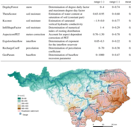
Table 2.Eight global mHM parameters (dimensionless): function, value range for FAST, range and arithmetic mean of sensitivity values (TEDPAS) across 14 Ruhr headwater catchments (1997–2006).

Parameter Process Description Value Sensitivity Sensitivity

range (–) range (–) mean (–)

DegdayForest snow Determination of degree daily factor 0–4 0–0.74 0.012

and maximum degree-day factor

ThetaSconst soil moisture Estimation of water content at 0.65–0.95 0–0.68 0.018

saturation of soil (constant part)

Ksconst soil moisture Estimation of saturated −1.9–0.0 0–0.77 0.392

vertical hydraulic conductivity

InfilShapeFactor soil moisture Determination of numerical 1–4 0–0.29 0.017

index of rooting distribution

AspectcorrPET meteo correction Account for aspect dependent 0.70–1.50 0–0.78 0.138

correction of PET

ExpslowInterflow interflow Determination of exponent 0.05–0.3 0–0.22 0.062

for the interflow reservoir

RechargeCoeff percolation Determination of percolation 0–70 0–0.38 0.057

coefficient

GeoParam baseflow Determination of baseflow 0–1000 0–0.47 0.012

recession parameter

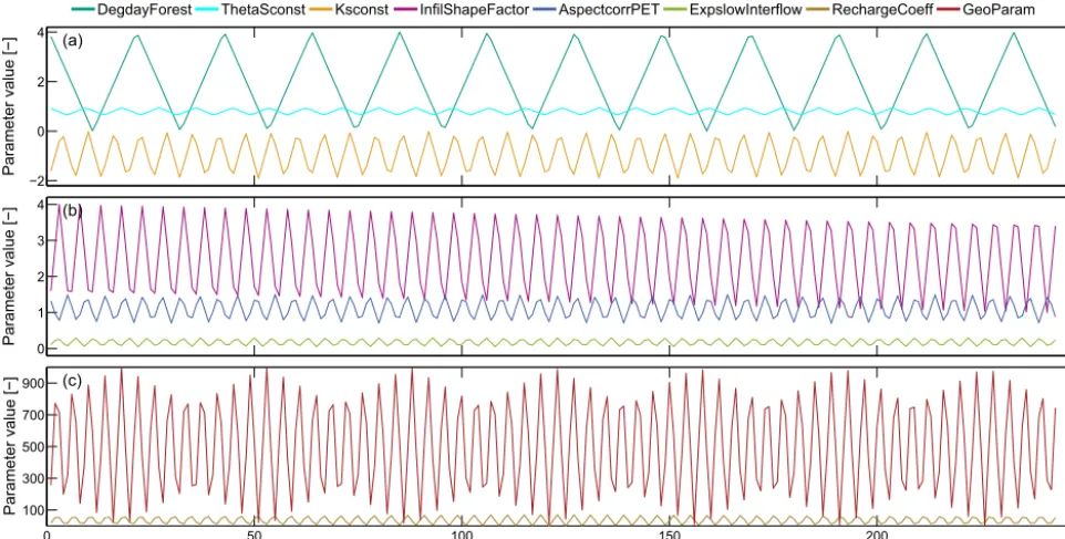
Figure 1. The Ruhr catchment with altitudinal zones, river network and 14 gauged headwater catchments: Amecke (AME), Bamenohl (BAM), Börlinghausen (BOE), Herrntrop (HER), Hüppcherhammer (HUE), Kickenbach (KIC), Kraghammer (KRA), Meschede1 (MES), Möhnesee-Neuhaus (MOE), Nichtinghausen (NIC), Olpe (OLP), Rüblinghausen (RUE), Völlinghausen (VOE), and Wenholthausen (WEN).

2.6 Study area and data

2.6.1 The Ruhr headwater catchments

The Ruhr (Fig. 1) has a catchment area of 4485 km2, and originates from a spring at about 670 m a.s.l. on the north-ern slope of the Ruhrkopf (842 m a.s.l.). The Ruhr joins the Rhine at Duisburg-Ruhrort (20 m a.s.l.) after 219 km. The landscape characteristics of the catchment range from densely wooded and scarcely populated lower mountain ranges in the Sauerland to widely sealed urban areas in the

−2 0 2 4

Parameter value [−]

(a)

0 1 2 3 4

Parameter value [−]

(b)

0 50 100 150 200 250

100 300 500 700 900

Parameter value [−]

(c)

Model run parameter set

DegdayForest ThetaSconst Ksconst InfilShapeFactor AspectcorrPET ExpslowInterflow RechargeCoeff GeoParam

Figure 2. (a–c)Variations of the eight selected global mHM parameters for 243 model runs with independent frequencies according to the FAST sampling plotted as connected curves (see also Table 2).

barrages, withdrawals, inlets) supplies almost 5 million peo-ple with drinking and processing water along the Ruhr, within its catchment and to adjacent watersheds.

Our investigations concentrate on 14 headwater catch-ments (Fig. 1) of the Ruhr River and its tributaries (e.g. Bigge, Lenne, and Möhne), where the hydrological regimes are much less affected by water management measures. The headwaters are situated in the eastern, rural part of the Ruhr basin with higher altitudes, and cover an area of 1742 km2 in total. Individual catchment sizes range from 28.7 km2 at gauge Amecke (AME) to 453.1 km2 at gauge Bamenohl (BAM). Average catchment slopes vary between 10.8 % (Rüblinghausen, RUE) and 26.1 % (Kickenbach, KIC). The dominant form of land cover is forest (39.7–87.3 %) followed by pasture (0.8–47.5 %), cropland (7.6–43.9 %) plus a few predominantly dispersed settlements (0.0–13.2 %; Table 3). The climatic conditions are humid warm-temperate (Göppert et al., 1998) with warm summers and moderate winters. An-nual mean temperature ranges between 8.45 and 5.45◦C at the lower and higher altitudes in the study area, respectively. Annual precipitation ranges from 1025 mm in the northeast to 1425 mm in the southwest (1997–2006; Table 3).

2.6.2 Data

Different kinds of observation data were used to set up and calibrate the hydrological model, to perform simulations for sensitivity analysis, and to derive the fingerprint metrics and a set of physiographic catchment descriptors.

Meteorological input data were daily values for precipita-tion (HYRAS; Rauthe et al., 2013), temperature (HYRAS; Frick et al., 2014), and potential evapotranspiration (AM-BAV; Löpmeier, 1994), all at a spatial resolution of 1 km2. Streamflow observations were available for all headwater catchments from 2002 to 2006. Spatial physiographic data were a digital elevation model (50 m×50 m), CORINE land cover data (100 m×100 m; European Environment Agency, 2009), a soil map (1 : 200 000; Bundesanstalt für Geowissenschaften und Rohstoffe, 2015a), and a geologi-cal map (1 : 1 000 000; Bundesanstalt für Geowissenschaften und Rohstoffe, 2015b).

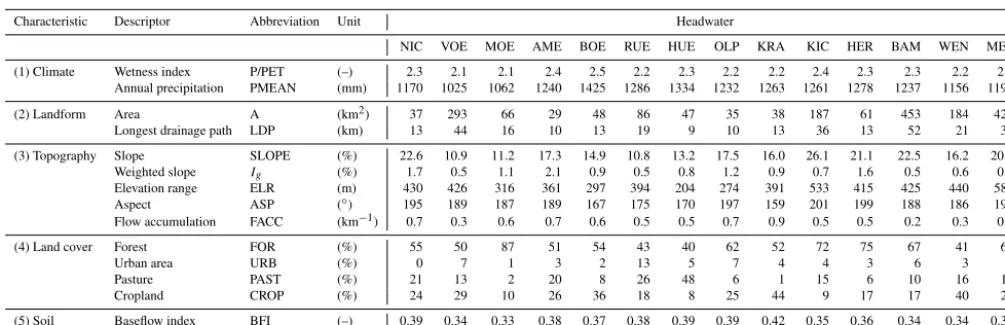
Table 3.Physiographic and climate descriptors characterising the topographic and hydroclimatic (1997–2006) setting of 14 Ruhr headwater catchments.

Characteristic Descriptor Abbreviation Unit Headwater

NIC VOE MOE AME BOE RUE HUE OLP KRA KIC HER BAM WEN MES

(1) Climate Wetness index P/PET (–) 2.3 2.1 2.1 2.4 2.5 2.2 2.3 2.2 2.2 2.4 2.3 2.3 2.2 2.5 Annual precipitation PMEAN (mm) 1170 1025 1062 1240 1425 1286 1334 1232 1263 1261 1278 1237 1156 1192

(2) Landform Area A (km2) 37 293 66 29 48 86 47 35 38 187 61 453 184 426 Longest drainage path LDP (km) 13 44 16 10 13 19 9 10 13 36 13 52 21 39

(3) Topography Slope SLOPE (%) 22.6 10.9 11.2 17.3 14.9 10.8 13.2 17.5 16.0 26.1 21.1 22.5 16.2 20.9 Weighted slope Ig (%) 1.7 0.5 1.1 2.1 0.9 0.5 0.8 1.2 0.9 0.7 1.6 0.5 0.6 0.7 Elevation range ELR (m) 430 426 316 361 297 394 204 274 391 533 415 425 440 585 Aspect ASP (◦_{) 195 189 187 189 167 175 170 197 159 201 199 188 186 190} Flow accumulation FACC (km−1) 0.7 0.3 0.6 0.7 0.6 0.5 0.5 0.7 0.9 0.5 0.5 0.2 0.3 0.2

(4) Land cover Forest FOR (%) 55 50 87 51 54 43 40 62 52 72 75 67 41 60

Urban area URB (%) 0 7 1 3 2 13 5 7 4 4 3 6 3 5

Pasture PAST (%) 21 13 2 20 8 26 48 6 1 15 6 10 16 10

Cropland CROP (%) 24 29 10 26 36 18 8 25 44 9 17 17 40 24

(5) Soil Baseflow index BFI (–) 0.39 0.34 0.33 0.38 0.37 0.38 0.39 0.39 0.42 0.35 0.36 0.34 0.34 0.31

characteristics and temporally aggregated fingerprint metrics introduced in Sect. 2.1.

3 Results

3.1 Temporal dynamics of parameter sensitivity (TEDPAS)

TEDPAS analysis for the 14 headwaters in the period of 1997–2006 showed a strong temporal dependence of the fraction of the total variance explainable by first-order sen-sitivities for hydrograph simulation. The sum of all eight pa-rameter sensitivity values per time step ranged between 0.26 and 0.87, while the average sum of the eight sensitivity val-ues per time step was 0.71. The spread between the maximal and minimal sum per time step was found to be smaller in the southwestern (e.g. Rüblinghausen RUE, 0.48) than in the northeastern (e.g. Völlinghausen VOE, 0.61) headwaters.

Minimal and maximal (sensitivity range) and the aver-age (sensitivity mean) sensitivity values of the eight parame-ters, summarised across all headwaters (Table 2), give a first impression that the soil moisture parameter Ksconst gener-ally exhibited the highest influence (sensitivity mean 0.392), while AspectcorrPET showed the largest range (sensitivity range 0–0.78). The interflow parameter ExpslowInterflow had the smallest sensitivity range (0–0.22), whereas parame-ters for snow (DegdayForest) and baseflow (GeoParam) had the overall lowest sensitivity mean values of 0.012. Across all headwaters, the parameters listed in terms of their average sensitivity to streamflow simulations are (in descending or-der): Ksconst, AspectcorrPET, ExpslowInterflow, Recharge-Coeff, ThetaSconst, InfilShapeFactor, GeoParam, and Deg-dayForest.

TEDPAS did not reveal many differences between the headwaters. For instance, Ksconst consistently had a highly dynamic course of sensitivity with frequently high values (Fig. 3a and b). Nevertheless, some of the parameters showed

differences between the headwaters, for example for Deg-dayForest (January–March; Fig. 3a and b) and Aspectcor-rPET (November–April; Fig. 3c and d). AspectcorAspectcor-rPET al-lows us to include the aspect of slopes, controlling insula-tion, in evapotranspiration estimations, while DegdayForest is a parameter related to snow dynamics in forested areas.

The example of these two parameters also illustrates the seasonality in sensitivity dynamics. AspectcorrPET showed highest sensitivity in the summer period from April to August, when evapotranspiration processes dominate and streamflow dynamics are low (Fig. 3c and d, g and h). Dur-ing that period, the parameter showed an alternatDur-ing course of sensitivity compared to Ksconst (Fig. 3b and d) with local maxima connected to (simulated) streamflow peaks (Fig. 3h). Higher sensitivities of DegdayForest were found for pe-riods (e.g. February) when snow processes (accumulation and melting) can occur. This was predominantly observed in catchments at higher altitudes – for example, for the headwa-ter VOE (up to 630 m a.s.l.) rather than for RUE (450 m a.s.l.; Fig. 3a and b). Also, VOE (50 %) exhibits a higher per-centage of forest cover (FOR) than RUE (43 %; Table 3). A similar distinction between summer and winter patterns was found for InfilShapeFactor, although at lower sensitivity lev-els (Fig. 3c and d). For the rest of the parameters either no seasonal patterns (e.g. RechargeCoeff; Fig. 3e and f) could be seen or only very low sensitivity values were found (e.g. ThetaSconst; Fig. 3a and b).

The ensembles of simulated streamflow compared reason-ably well with the observed hydrographs (Fig. 3g and h), al-though the simulation ensemble underestimated some high-flow periods.

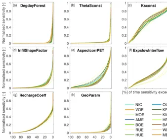
3.2 Sensitivity duration

0 0.2 0.4 0.6 0.8 _{(a) RUE}

Sensitivity [−]

0 0.2 0.4 0.6 0.8 _{(b) VOE}

0 0.2 0.4 0.6 0.8 _(c)

Sensitivity [−]

0 0.2 0.4 0.6 0.8 _(d)

0 0.2 0.4 0.6 0.8 _(e)

Sensitivity [−]

0 0.2 0.4 0.6 0.8 _(f)

2 8 14 20 (g)

Q

[m

³ s

-1]

Nov 2002Dec 2002 Jan 2003Feb 2003Mar 2003 Apr 2003May 2003Jun 2003 Jul 2003Aug 2003Sep 2003 Oct 2003

5 15 25 35 (h)

Nov 2002Dec 2002 Jan 2003Feb 2003Mar 2003 Apr 2003May 2003Jun 2003 Jul 2003Aug 2003Sep 2003 Oct 2003

DegdayForest ThetaSconst Ksconst DegdayForest ThetaSconst Ksconst

InfilShapeFactor AspectcorrPET ExpslowInterflow InfilShapeFactor AspectcorrPET ExpslowInterflow

RechargeCoeff GeoParam RechargeCoeff GeoParam

Observed Simulated Observed Simulated

Figure 3.Time-dependent FAST sensitivities (TEDPAS) of eight global mHM parameters for two headwater gauges RUE(a, c, e)and VOE(b, d, f), and observed and FAST-mHM simulated streamflow ensembles at gauges RUE(g)and VOE(h). The results are shown for the hydrological year 2003 consisting of a wet season (November 2002–March 2003) and a long dry period from April 2003 to September

2003. Please note the different axis scaling for streamflow for the two headwaters(g, h).

the parameters, with either very low (e.g. DegdayForest; Fig. 4a and ThetaSconst; Fig. 4b), intermediate (Recharge-Coeff; Fig. 4g) or high (Ksconst; Fig. 4c) influence with re-spect to sensitivity exceedance probability.

Some of the parameters showed a regional variation of SDCs. Four of eight parameters, i.e. Ksconst (Fig. 4c), In-filShapeFactor (Fig. 4d), AspectcorrPET (Fig. 4e), and Ex-pslowInterflow (Fig. 4f), revealed certain differences among the headwaters. The SDCs of the two most influential param-eters Ksconst (Fig. 4c) and AspectcorrPET (Fig. 4e) showed a systematic spread for the different headwaters, with the curve of gauge RUE plotting at the lower (Fig. 4c) and upper (Fig. 4e) margins of the group of headwaters, respectively. For InfilShapeFactor (Fig. 4d), the headwater Möhnesee-Neuhaus (MOE), and for ExpslowInterflow (Fig. 4f) both RUE and MOE deviated from the other headwaters and showed lower SDC values.

In the case of AspectcorrPET (Fig. 4e), the SDCs were sorted from the southwestern (e.g. RUE) to the northeastern (e.g. MES) headwaters (Fig. 1). In the southwestern headwa-ters (e.g. RUE) the slopes are gentler with lower relief en-ergy than further northeast, where valleys are more deeply incised (e.g. NIC, SLOPE and ELR; Table 3). The slopes in the southwestern headwaters are on average facing southeast, compared to the more southwest-facing slopes in the north-ern and eastnorth-ern Ruhr headwaters (ASP; Table 3). Besides showing a different aspect, the southwestern headwater RUE

also has the highest proportion of urban areas (URB, 13 %; Table 3). Both factors influence the estimation of evapotran-spiration in mHM and hence streamflow simulations.

The SDCs of the most sensitive parameter Ksconst (Fig. 4c) showed concave curvatures, in contrast to the other parameters which had convex SDCs. The SDCs of the largest headwater Bamenohl (BAM) fell in between the other catch-ments, showing a kind of transitional behaviour of sensitivity duration (Fig. 4), except for ExpslowInterflow.

3.3 Parameter sensitivity to fingerprints (INDPAS) 3.3.1 Single-value indices

Similar patterns of parameter sensitivities to single-value fin-gerprints were consistently found across all 14 headwaters. Figure 5 shows the matrix representations for four represen-tative headwaters (RUE, VOE, HER, and WEN). All of them comprise eight rows for the parameters and eight columns for the fingerprint metrics. Sensitivity to a specific fingerprint is arranged column-wise.

con-Figure 4.Sensitivity duration curves (SDCs) for eight global mHM parameters of 14 Ruhr headwater catchments (1997–2006):

DegdayFor-est(a), ThetaSconst(b), Ksconst(c), InfilShapeFactor(d), AspectcorrPET(e), ExpslowInterflow(f), RechargeCoeff(g), and GeoParam(h).

SDCs are shown normalised by the highest sensitivity value for each parameter among the headwaters. The eight parameters in terms of their average importance to streamflow simulations (TEDPAS) among all headwaters listed in descending order: Ksconst, AspectcorrPET, ExpslowInterflow, RechargeCoeff, ThetaSconst, InfilShapeFactor, GeoParam, and DegdayForest.

trast, AspectcorrPET was the most sensitive parameter, while others, including Ksconst, showed almost no sensitivity to the simulation of the overall water balance. The parame-ters RechargeCoeff and Ksconst had similarly highest impor-tance for the simulation of the fingerprint SLFDC (slope of the flow duration curve). Other parameter–fingerprint com-binations revealed parameters with very low sensitivity val-ues, e.g. DegdayForest or GeoParam, which showed very low sensitivities to all of the eight fingerprint metrics (Fig. 5).

Only minor differences in these patterns occurred between the catchments, and these related to small deviations in abso-lute sensitivity values or in the order of the second and third rank, e.g. for the fingerprint ACT (Fig. 5).

3.3.2 Flow duration curve

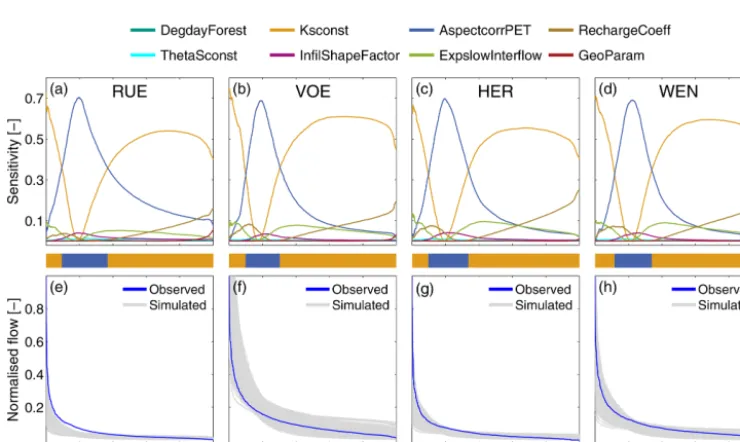
Using FDCs as model response targets revealed parame-ter sensitivities to different streamflow magnitudes. Again, a high proportion of similarities among the headwaters was found. The highest influence was alternately exerted by the parameters Ksconst and AspectcorrPET (Fig. 6a–d); their courses of parameter sensitivity were highly anticorrelated (mean correlation across all headwaters r= −0.975). The soil moisture parameter Ksconst clearly dominated the very

high flows (0–10 % of time Qis exceeded) and the entire mid- and low-flow sections (40–100 %); moderate high flows between 10 and 40 % were most affected by changes in the evapotranspiration parameter AspectcorrPET. These changes in the dominating parameter are additionally illustrated in Fig. 6 by a catchment-specific strip showing the pattern of parametric dominance along the FDC, which showed only slight differences in the lengths of the intermittent parts (As-pectcorrPET) between the headwaters.

Figure 5.Sensitivity of eight global mHM parameters to eight single-value fingerprint metrics (RR, CV, HPC, SLFDC, HFD, BFI, RTC,

ACT) in four Ruhr headwater catchments: RUE(a), VOE(b), HER(c), WEN(d). The simulation period was 1997 to 2006.

Figure 6. (a–d)Sensitivity of eight global mHM parameters along streamflow exceedance probability (flow duration curve, FDC) for four Ruhr headwater catchments RUE, VOE, HER, and WEN. Catchment-specific strips show the parameters with the highest sensitivity along

the FDC.(e–h)Observed flow duration curves and the corresponding ensembles of each 243 simulated FDCs for the period 2002 to 2006,

Interestingly, the ensembles of normalised FDCs showed distinct differences between the catchments (Fig. 6e–h), al-though the sensitivity dynamics were similar, and the same 243 parameter variations from FAST were used for each headwater. The largest spread of FDCs was found for the northeastern headwater VOE (Fig. 6f) with the largest catch-ment size among the four shown headwaters. The smaller headwaters WEN, HER, and RUE (Fig. 1) showed a decreas-ing spread of the FDCs from northeast to southwest (Fig. 6h, g, e). Additionally, the widths of the simulation envelopes changed for different streamflow magnitudes. All ensembles of FDCs showed a constriction point located at about 20 % of streamflow exceedance (Fig. 6e–h), which is the same point where Ksconst and AspectcorrPET showed lowest and highest sensitivity values, respectively (Fig. 6a–d). The en-sembles of simulated FDCs encompassed the observed FDC in most cases (e.g. VOE, HER, WEN; Fig. 6f–h). In some cases the observed FDC was outside the simulated range (e.g. RUE; Fig. 6e).

4 Discussion

4.1 Parameter sensitivities from TEDPAS and INDPAS The combination of TEDPAS and INDPAS created a detailed sensitivity pattern for the response characteristics of the hy-drological model mHM. Overall, the soil moisture dynamics parameter Ksconst and the evapotranspiration parameter As-pectcorrPET were found most relevant for the simulation of the streamflow response of 14 Ruhr headwaters.

The TEDPAS analysis confirmed, as expected, a season-ality of sensitivity for parameters controlling snow (Deg-dayForest) or evapotranspiration (AspectcorrPET) processes. More interestingly, TEDPAS also showed an alternating dominance of Ksconst and AspectcorrPET during the tem-poral course of the simulation. Using flow duration curves as response targets (INDPAS) clarified that this was related to different streamflow magnitudes. The soil moisture dynamics (Ksconst) dominated at both high and low flows, which may be attributed to the dual role of Ksconst in parameterising both storage (field capacity) and transmission (conductivity) of soil water in mHM. During intermediate-flow conditions, evapotranspiration (AspectcorrPET) governed the stream-flow simulations, probably because of the high influence of evapotranspiration on the shallow soil storage and thus the system state of the catchment. This high sensitivity of an evapotranspiration parameter during intermediate-flow con-ditions coincides with the findings of former studies (e.g. Guse et al., 2014, 2016b).

The specific influence of AspectcorrPET was mainly on the water balance (fingerprint RR) in all of the headwaters. Ksconst was the most sensitive parameter for most of the other single-value fingerprints, encompassing those quanti-fying low-flow (BFI) as well as high-flow conditions or the

flashiness of hydrological response (CV, HPC, HFD, RTC). Only for one single-value fingerprint (SLFDC, related to the rate of change in streamflow) another parameter (Recharge-Coeff) was found to be as sensitive as Ksconst. The moder-ate relevance of the groundwmoder-ater-relmoder-ated RechargeCoeff in-creased during low-flow periods, as illustrated by INDPAS using FDCs and TEDPAS.

A temporally resolved sensitivity makes it difficult to re-veal clear patterns of dominant parameters when dealing with long time periods. Guse et al. (2016b) also recognised that parameter sensitivity by TEDPAS based on the streamflow hydrograph should be analysed on different temporal aggre-gation levels and should be related to different streamflow magnitudes for a detailed assessment of dominant model parameters and temporal process dynamics. While their methodological approach was purely based on aggregation and reordering of TEDPAS sensitivity and streamflow time series, we added additional value with INDPAS aiming at multiple response targets including FDCs. The consideration of flow duration curves enabled analysing streamflow free of autocorrelation and time dependence. The FDC as a model response target for sensitivity analysis provided information on parameter sensitivity along the independent variable of streamflow exceedance probability. In contrast, for classical hydrograph inspection, which is the basis of TEDPAS, time is the independent variable. INDPAS along FDCs allowed us to draw conclusions about parametric influences at specific streamflow magnitudes.

Regardless of the chosen model response target, in the case of 14 Ruhr headwaters only one or a very small group of pa-rameters were identified as relevant for streamflow response. In this context, Herman et al. (2013) showed that the long-term water balance is dominated by only very few param-eters, irrespective of the hydrological conditions and of the model. Cuntz et al. (2015) performed a global Sobol sensitiv-ity analysis on the hydrologic model mHM. For three distinct humid and arid European catchments this analysis always re-sulted in about 20 informative parameters, though the dom-inant parameter sets were composed very differently. Their criteria to select the sensitive parameters was substantially different from our approach, which renders a direct compar-ison between the studies difficult. The different number of dominant parameters might also be due to correlated mHM parameters which we sorted out before sensitivity analysis. In contrast, Cuntz et al. (2015) considered the degree of cor-relation between mHM parameters as rather minor to be in-terfering with parameter identification.

the parameter space and need for constraining parameter val-ues and thus facilitates model calibration. A missing sensi-tivity signal to a fingerprint (e.g. RechargeCoeff to RR) can reveal that the chosen response target might not be relevant to further constrain the parameter identification in a certain catchment.

The spread of the simulated response ensembles allows us to judge whether a fingerprint metric is a reliable re-sponse target for sensitivity analysis or whether different fin-gerprints, e.g. the master recession curve or the double mass curve, should be considered instead. For example, the hy-drographs and FDCs showed significant spread that also dif-fered between the catchments (Figs. 3 and 6). In contrast, the spread in simulated values for the Autocorrelation Time (ACT) was small for all catchments. Accordingly, INDPAS analysis directed to ACT also showed only moderate sensi-tivities for the set of eight parameters (Fig. 5). Our preselec-tion of eight parameters can potentially lead to the elimina-tion of other storage parameters that might be most sensitive to ACT. Thus, one might conclude that parameter selection based on INDPAS would result in a different choice in the set of the most sensitive parameters. In the case of ACT this is not very likely, since storage parameters (e.g. ExpslowInter-flow and GeoParam) were still included. Instead, the precip-itation time series has a large impact on the autocorrelation structure of streamflow; the ACT metric is thus less informa-tive than others that depend less on the hydroclimatic bound-ary conditions.

The resulting partial variances for each fingerprint are comparable as they portray the relative influence of the pa-rameters on the variation of the target, regardless of the spe-cific values of the targets. In order to take into account the im-pact of the spread of the simulation results on the parameter sensitivities, a weighting factor for partial parameter sensitiv-ities might be helpful. An impact-weighted INDPAS might then be used along with catchment class-specific response fingerprints to select relevant parameters for the specific hy-drological conditions. In Fig. 6 we normalised the FDCs by the maximum value of each time series. For the visual com-parison of sites this is a necessary step, but it might lead to a different form of appearance, including the spread of the sim-ulation ensemble. If absolute fingerprint values are replaced by normalised quantities (Samaniego et al., 2010a; He et al., 2011), dimensions should be considered explicitly when de-termining sensitivity weighting factors.

Our findings using different model response targets con-firm the necessity of a multivariate sensitivity analysis. This was similarly recognised by Wagener et al. (2009), who ap-plied three standard error metrics as objective functions for sensitivity analysis. Their results for parameter sensitivity were found to change spatially when the objective function was replaced. Razavi and Gupta (2015) similarly pointed out that even conflicting conclusions could be drawn if different properties of the model response were applied in sensitiv-ity analysis. To avoid misinterpretation of sensitivsensitiv-ity results

we propose that the selection of specific fingerprint metrics should be determined by the purpose of the modelling; for instance, sensitivity to fingerprint metrics for peak flow is suitable if flood prediction is the focus. Redundancy is not problematic if several similar metrics for a specific stream-flow characteristic are selected, e.g. HPC, CV, and HFD for high flows. A multivariate analysis with metrics of several, even partly similar streamflow characteristics (frequency of high flow, magnitude of high flows etc.) is rather helpful to ensure complete parameter identification for different catch-ments. Aggregated and temporally independent fingerprints like the FDC proved to be especially applicable.

4.2 Regional differences in parameter sensitivity Although the most sensitive parameters and the correspond-ing sensitivity patterns of streamflow response were found to be similar for the 14 investigated Ruhr headwater catch-ments, the analysis with TEDPAS and INDPAS revealed cer-tain regional differences.

Especially the analysis of sensitivity duration curves de-rived from TEDPAS revealed regional differences of param-eter sensitivity between headwaters. For half of the eight selected parameters we found regional differences in SDCs (Sect. 3.2 and Fig. 4). The most sensitive parameters exhib-ited the largest spread of SDCs (e.g. Ksconst and Aspect-CorrPET; Fig. 4c and e), and their SDCs were systematically ordered according to the geographical location (southwest– northeast) and the physiographic setting (ASP, URB; Ta-ble 3). Some catchments deviate from the general pattern in SDCs for evapotranspiration and interflow parameters (e.g. RUE; Fig. 4e and f). In these cases, the specific combina-tion of catchment characteristics (degree of soil sealing, to-pographic gradients, land cover) might have led to different processes in streamflow simulations. For the catchment of RUE, the smallest slope value among the headwaters in con-junction with the highest percentage of urban area (SLOPE, URB; Table 3) can explain the deviation from the general pattern of SDCs for the two parameters. SDCs thus provided a convenient means to identify regionally different sensitivity characteristics for each of the analysed parameters.

The results from the INDPAS analysis directed to single-valued fingerprints also showed some differences between the headwaters. In particular, the sensitivity patterns of the second and third ranked parameters were found to differ, although not with the same systematic ordering as for the SDCs. The patterns of the most sensitive parameters along streamflow exceedance probability (catchment-specific strips in Fig. 6) provided visually condensed diagnostic informa-tion for different streamflow magnitudes, but showed only minor differences between the catchments.

(2014), who reported almost no differences of parameter sen-sitivities among different subcatchments of the Treene in northern Germany in a similar analysis. This was explained by the absence of a pronounced heterogeneity in their study area.

Given that the same parameter sets are applied to all head-water catchments, any regional differences in parameter sen-sitivity originate from differences either in the hydroclimatic or in the physiographic setting. In the case of the Ruhr headwaters, the local hydroclimatic and physiographic dif-ferences (Table 3) seem to be sufficient to be discriminated by the hydrological model structure in the form of a differ-ent variation in streamflow response. Due to their geograph-ical proximity, the 14 Ruhr headwaters are generally similar in terms of the long-term hydroclimate (Wetness Index) and the physiography, e.g. in their soil hydrological characteris-tics (BFI). They show, however, some differences in annual precipitation amount, topographic gradient, and land cover. The average annual precipitation in the simulation period be-tween 1997 and 2006 reveals a hydroclimatic gradient with lower to higher precipitation rates from northeast to south-west (PMEAN), similar to the geographical ordering of the SDCs in Fig. 4. Song et al. (2013) also attributed local dif-ferences of parameter sensitivity to the spatial distribution of meteorologic forcing. Demaria et al. (2007) similarly con-cluded that parameter sensitivity was more strongly deter-mined by climate gradients than by changes in soil properties in their Monte Carlo-based sensitivity study. Under differ-ent hydrological conditions, regional sensitivity patterns or the number of parameters which influence streamflow simu-lations might be different from the present example (Cuntz et al., 2015).

As parameter sensitivity is a prerequisite for parameter identifiability, even slight differences in sensitivity reveal in-formation about how identifiability can change among differ-ent catchmdiffer-ents. Scale-dependdiffer-ent limitations have to be kept in mind to avoid a levelling out of the explanatory value of a physiographic descriptor (Blöschl and Sivapalan, 1995), pos-sibly resulting in an intermediate course of sensitivity dura-tion as seen for the largest headwater of Bamenohl (BAM; Sect. 3.2 and Fig. 4). van Griensven et al. (2006) remarked that local differences indicate that results of global sensitiv-ity analysis for one catchment cannot be directly applied to other, even nearby locations, but may be used as reason-able estimates within the same catchment category. Loca-tions with intermediate-sensitivity characteristics (e.g. BAM) could at least serve as a starting point for parameter trans-fer to closely located ungauged sites. As the local diftrans-fer- differ-ences between the Ruhr headwaters are not very large, the most sensitive parameters found for WEN in the first step of the analysis with all model parameters were also domi-nant in the other subcatchments, which was corroborated by the TEDPAS analysis with eight selected parameters on all subcatchments. Any local differences in parameter sensitiv-ity revealed by the analysis of sensitivsensitiv-ity duration or INDPAS

could then be handled during individual model calibration for each catchment.

5 Conclusions

We used FAST for a global sensitivity analysis of the hy-drological model mHM in 14 headwater catchments of the Ruhr River in Germany. Our multilevel approach not only reveals the dominating parameters for streamflow simulation but also pinpoints the influences of the analysed parameters to diverse aspects of hydrological response processes. Espe-cially the application of several hydrological fingerprints as response targets allows for detailed model diagnostics. Com-parison of streamflow response characteristics and analysing along the range of streamflow magnitudes shows how the parametric dominances and the most influential parameters can change with streamflow conditions, for example the com-plementary sensitivity of soil moisture dynamics and evapo-transpiration in our case. The combination of TEDPAS and INDPAS also provides a means to unveil the slight differ-ences in catchment-specific patterns between the closely lo-cated headwaters. The general similarity in the sensitivity patterns indicates, however, that a parameter transfer to other catchments might be possible, provided that the interplay of catchment structure and local hydroclimate has evolved in a similar way.

Data availability. The streamflow data and the digital elevation model used in this study are not publicly accessible, and were pro-vided by the Ruhrverband in Essen.

The further spatial physiographic data can be downloaded from the web: land cover data (https://land.copernicus.eu/

pan-european/corine-land-cover/clc-2006?tab=download); soil

data (https://produktcenter.bgr.de/terraCatalog/OpenSearch.do?

search=3E80DA1A-A9A7-45A3-9CC7-79796FE9ABA4&type=

/Query/OpenSearch.do); geological data (https://

produktcenter.bgr.de/terraCatalog/DetailResult.do?fileIdentifier= 1C60DDA9-EF73-47B9-9ED7-FCD22B3226C1).

Meteorological input data are available from Deutscher Wet-terdienst. Data for precipitation (HYRAS; Rauthe et al., 2013) and temperature (HYRAS; Frick et al., 2014) can be obtained via https://www.dwd.de/DE/leistungen/hyras/hyras.html. The database for potential evapotranspiration (AMBAV; Löpmeier, 1994) can be accessed via ftp://ftp-cdc.dwd.de/pub/CDC/grids_germany/daily/ evapo_p.

Competing interests. The authors declare that they have no conflict of interest.

Acknowledgements. The streamflow data and the digital elevation model used in this study were provided by the Ruhrverband in Essen. We thank Linda Bergmann, who supported the techni-cal implementation of the FAST analysis. We are grateful to Fanny Sarrazin, Sibylle Haßler, Björn Guse, Shervan Gharari, and one anonymous reviewer for their critical comments on this and an earlier version of the manuscript, which greatly helped to improve the paper. We acknowledge support by Deutsche Forschungsgemeinschaft and Open Access Publishing Fund of Karlsruhe Institute of Technology.

The article processing charges for this open-access publication were covered by a Research

Centre of the Helmholtz Association.

Edited by: Ross Woods

Reviewed by: Björn Guse and Shervan Gharari

References

Atkinson, S. E., Sivapalan, M., Woods, R. A., and Viney, N. R.: Dominant physical controls on hourly flow predictions and the role of spatial variability: Mahurangi catchment, New Zealand, Adv. Water Res., 26, 219–235, https://doi.org/10.1016/S0309-1708(02)00183-5, 2003.

Beven, K.: Prophecy, reality and uncertainty in distributed

hydrological modelling, Adv. Water Res., 16, 41–51,

https://doi.org/10.1016/0309-1708(93)90028-E, 1993.

Beven, K.: How far can we go in distributed

hydrolog-ical modelling?, Hydrol. Earth Syst. Sci., 5, 1–12,

https://doi.org/10.5194/hess-5-1-2001, 2001.

Black, P.: Watershed functions, J. Am. Water Resour. Assoc., 33, 1–11, 1997.

Blöschl, G. and Sivapalan, M.: Scale issues in hydrolog-ical modelling: A review, Hydrol. Process., 9, 251–290, https://doi.org/10.1002/hyp.3360090305, 1995.

Bode, H., Evers, P., and Albrecht, D. R.: Integrated water resources management in the Ruhr River Basin, Germany, Water Sci. Tech-nol., 47, 81–86, 2003.

Brudy-Zippelius, T.: Wassermengenbewirtschaftung im Einzugsge-biet der Ruhr : Simulation und Echtzeitbetrieb, PhD thesis, Uni-versität Karlsruhe (TH), 159 pp., 2003.

Bundesanstalt für Geowissenschaften und Rohstoffe:

Bo-denübersichtskarte der Bundesrepublik Deutschland 1:200.000 (BÜK200), 2015a.

Bundesanstalt für Geowissenschaften und Rohstoffe: Geologische Karte der Bundesrepublik Deutschland 1:1000000 (GK1000), 2015b.

Castiglioni, S., Lombardi, L., Toth, E., Castellarin, A.,

and Montanari, A.: Calibration of rainfall-runoff

mod-els in ungauged basins: A regional maximum

like-lihood approach, Adv. Water Res., 33, 1235–1242,

https://doi.org/10.1016/j.advwatres.2010.04.009, 2010. Cibin, R., Sudheer, K. P., and Chaubey, I.: Sensitivity and

identifiability of stream flow generation parameters of

the SWAT model, Hydrol. Process., 24, 1133–1148,

https://doi.org/10.1002/hyp.7568, 2010.

Clark, M. P., McMillan, H. K., Collins, D. B. G., Kavetski, D., and Woods, R. A.: Hydrological field data from a modeller’s perspec-tive: Part 2: Process-based evaluation of model hypotheses, Hy-drol. Process., 25, 523–543, https://doi.org/10.1002/hyp.7902, 2011.

Cloke, H. L., Pappenberger, F., and Renaud, J.-P.: Multi-Method Global Sensitivity Analysis (MMGSA) for modelling flood-plain hydrological processes, Hydrol. Process., 22, 1660–1674, https://doi.org/10.1002/hyp.6734, 2008.

Cukier, R. I., Fortuin, C. M., Shuler, K. E., Petschek, A. G., and Schaibly, J. H.: Study of the sensitivity of coupled reaction sys-tems to uncertainties in rate coefficients. I Theory, J. Chem. Phys., 59, 3873, https://doi.org/10.1063/1.1680571, 1973. Cukier, R. I., Schaibly, J. H., and Shuler, K. E.: Study of the

sen-sitivity of coupled reaction systems to uncertainties in rate co-efficients. III. Analysis of the approximations Theory, J. Chem. Phys., 63, 1140, https://doi.org/10.1063/1.431440, 1975. Cuntz, M., Mai, J., Zink, M., Thober, S., Kumar, R., Schäfer,

D., Schrön, M., Craven, J., Rakovec, O., Spieler, D., Prykhodko, V., Dalmasso, G., Musuuza, J., Langenberg, B., Attinger, S., and Samaniego, L.: Computationally inexpen-sive identification of noninformative model parameters by sequential screening, Water Resour. Res., 51, 6417–6441, https://doi.org/10.1002/2015WR016907, 2015.

Demaria, E. M., Nijssen, B., and Wagener, T.: Monte Carlo sen-sitivity analysis of land surface parameters using the Vari-able Infiltration Capacity model, J. Geophys. Res., 112, 1–15, https://doi.org/10.1029/2006JD007534, 2007.

Di Prinzio, M., Castellarin, A., and Toth, E.: Data-driven catchment classification: application to the pub problem, Hydrol. Earth Syst. Sci., 15, 1921–1935, https://doi.org/10.5194/hess-15-1921-2011, 2011.

effec-tive precipitation identification, J. Hydrol., 150, 115–149, https://doi.org/10.1016/0022-1694(93)90158-6, 1993.

European Environment Agency: CORINE Land Cover (CLC2006), 2009.

Euser, T., Winsemius, H. C., Hrachowitz, M., Fenicia, F., Uhlen-brook, S., and Savenije, H. H. G.: A framework to assess the re-alism of model structures using hydrological signatures, Hydrol. Earth Syst. Sci., 17, 1893–1912, https://doi.org/10.5194/hess-17-1893-2013, 2013.

Farmer, D., Sivapalan, M., and Jothityangkoon, C.: Climate, soil, and vegetation controls upon the variability of water bal-ance in temperate and semiarid landscapes: Downward ap-proach to water balance analysis, Water Resour. Res., 39, 1035, https://doi.org/10.1029/2001wr000328, 2003.

Fontaine, D. D., Havens, P. L., Blau, G. E., and Tillotson, M.: Groundwater Risk Modeling for Pesticides, Weed Technol., 6, 716–724, 1992.

Frey, H. C. and Patil, S. R.: Identification and review of sen-sitivity analysis methods, Computat. Studies, 22, 553–578, https://doi.org/10.1111/0272-4332.00039, 2002.

Frick, C., Steiner, H., Mazurkiewicz, A., Riediger, U., Rauthe, M., Reich, T., and Gratzki, A.: Central European high-resolution gridded daily data sets (HYRAS): Mean temperature and relative humidity, Meteorol. Z., 23, 15–32, https://doi.org/10.1127/0941-2948/2014/0560, 2014.

Göppert, H., Ihringer, J., Plate, E. J., and Morgenschweis, G.: Flood forecast model for improved reservoir management in the Lenne River catchment, Germany, Hydrolog. Sci. J., 43, 215– 242, https://doi.org/10.1080/02626669809492119, 1998. Gupta, H. V., Sorooshian, S., and Yapo, P. O.: Toward improved

calibration of hydrologic models: Multiple and noncommensu-rable measures of information, Water Resour. Res., 34, 751–763, https://doi.org/10.1029/97WR03495, 1998.

Gupta, H. V., Wagener, T., and Liu, Y.: Reconciling the-ory with observations: elements of a diagnostic approach

to model evaluation, Hydrol. Process., 22, 3802–3813,

https://doi.org/10.1002/hyp.6989, 2008.

Gupta, H. V., Clark, M. P., Vrugt, J. A., Abramowitz, G., and Ye, M.: Towards a comprehensive assessment of model structural adequacy, Water Resour. Res., 48, 1–16, https://doi.org/10.1029/2011WR011044, 2012.

Guse, B., Reusser, D. E., and Fohrer, N.: How to improve the representation of hydrological processes in SWAT for a low-land catchment – temporal analysis of parameter sensitiv-ity and model performance, Hydrol. Process., 28, 2651–2670, https://doi.org/10.1002/hyp.9777, 2014.

Guse, B., Pfannerstill, M., Gafurov, A., Fohrer, N., and Gupta, H.: Demasking the integrated information of discharge: Advancing sensitivity analysis to consider different hydrological compo-nents and their rates of change, Water Resour. Res., 52, 8724– 8743, https://doi.org/10.1002/2016WR018894, 2016a.

Guse, B., Pfannerstill, M., Strauch, M., Reusser, D. E., Lüdtke, S., Volk, M., Gupta, H., and Fohrer, N.: On char-acterizing the temporal dominance patterns of model pa-rameters and processes, Hydrol. Process., 30, 2255–2270, https://doi.org/10.1002/hyp.10764, 2016b.

Hamby, D. M.: A review of techniques for parameter sensitivity analysis of environmental models, Environ. Monit. Assess., 32, 135–154, https://doi.org/10.1007/BF00547132, 1994.

He, Y., Bárdossy, A., and Zehe, E.: A catchment classification scheme using local variance reduction method, J. Hydrol., 411, 140–154, https://doi.org/10.1016/j.jhydrol.2011.09.042, 2011. Herman, J. D., Reed, P. M., and Wagener, T.: Time-varying

sen-sitivity analysis clarifies the effects of watershed model formu-lation on model behavior, Water Resour. Res., 49, 1400–1414, https://doi.org/10.1002/wrcr.20124, 2013.

Hogue, T. S., Sorooshian, S., Gupta, H., Holz, A.,

and Braatz, D.: A Multistep Automatic Calibration

Scheme for River Forecasting Models, J.

Hydrom-eteorol., 1, 524–542,

https://doi.org/10.1175/1525-7541(2000)001<0524:AMACSF>2.0.CO;2, 2000.

Kavetski, D. and Clark, M. P.: Ancient numerical daemons of conceptual hydrological modeling: 2. Impact of time stepping schemes on model analysis and prediction, Water Resour. Res., 46, 1–27, https://doi.org/10.1029/2009WR008896, 2010. Kirchner, J. W.: Getting the right answers for the right

rea-sons: Linking measurements, analyses, and models to ad-vance the science of hydrology, Water Resour. Res., 42, 1–5, https://doi.org/10.1029/2005WR004362, 2006.

Kumar, R., Samaniego, L., and Attinger, S.: The effects of spa-tial discretization and model parameterization on the predic-tion of extreme runoff characteristics, J. Hydrol., 392, 54–69, https://doi.org/10.1016/j.jhydrol.2010.07.047, 2010.

Kumar, R., Samaniego, L., and Attinger, S.: Implications of dis-tributed hydrologic model parameterization on water fluxes at multiple scales and locations, Water Resour. Res., 49, 360–379, https://doi.org/10.1029/2012WR012195, 2013.

Löpmeier, F.-J.: Berechnung der Bodenfeuchte und Verdun-stung mittels agrarmeteorologischer Modelle, Zeitschrift f. Be-wässerungswirtschaft, 29, 157–167, 1994.

Lu, Y. C. and Mohanty, S.: Sensitivity Analysis of a complex, pro-posed geological waste disposal system using the Fourier Ampli-tude Sensitivity Test Method, Reliab. Eng. Syst. Safe., 72, 275– 291, https://doi.org/10.1016/s0951-8320(01)00020-5, 2001. Massmann, C. and Holzmann, H.: Analysis of the behavior of

a rainfall-runoff model using three global sensitivity analysis methods evaluated at different temporal scales, J. Hydrol., 475, 97–110, https://doi.org/10.1016/j.jhydrol.2012.09.026, 2012. Massmann, C. and Holzmann, H.: Analysing the Sub-processes of a

Conceptual Rainfall-Runoff Model Using Information About the Parameter Sensitivity and Variance, Environ. Monit. Assess., 20, 41–53, https://doi.org/10.1007/s10666-014-9414-6, 2015. Massmann, C., Wagener, T., and Holzmann, H.: A new

ap-proach to visualizing time-varying sensitivity indices

for environmental model diagnostics across

evalua-tion time-scales, Environ. Modell. Softw., 51, 190–194, https://doi.org/10.1016/j.envsoft.2013.09.033, 2014.

McCuen, R. H.: The role of sensitivity analysis in hydrologic modeling, J. Hydrol., 18, 37–53, https://doi.org/10.1016/0022-1694(73)90024-3, 1973.

Nossent, J. and Bauwens, W.: Multi-variable sensitivity and identi-fiability analysis for a complex environmental model in view of integrated water quantity and water quality modeling, Water Sci. Technol., 65, 539–549, https://doi.org/10.2166/wst.2012.884, 2012.

O’Loughlin, F., Bruen, M., and Wagener, T.: Parameter sen-sitivity of a watershed-scale flood forecasting model as a function of modelling time-step, Hydrol. Res., 44, 334–350, https://doi.org/10.2166/nh.2012.157, 2013.

Pfannerstill, M., Guse, B., Reusser, D., and Fohrer, N.: Process verification of a hydrological model using a temporal parame-ter sensitivity analysis, Hydrol. Earth Syst. Sci., 19, 4365–4376, https://doi.org/10.5194/hess-19-4365-2015, 2015.

Pianosi, F. and Wagener, T.: Understanding the time-varying impor-tance of different uncertainty sources in hydrological modelling using global sensitivity analysis, Hydrol. Process., 30, 3991– 4003, https://doi.org/10.1002/hyp.10968, 2016.

Plate, E. J., Ihringer, J., and Lutz, W.: Operational models for flood calculations, J. Hydrol., 100, 489–506, 1988.

Poff, N. L., Allan, J. D., Bain, M. B., Karr, J. R., Prestegaard, K. L., Richter, B. D., Sparks, R. E., and Stromberg, J. C.: The Natural Flow Regime: A paradigm for river conservation and restoration N, BioScience, 47, 769–784, https://doi.org/10.2307/1313099, 1997.

Pokhrel, P., Yilmaz, K. K., and Gupta, H. V.: Multiple-criteria cal-ibration of a distributed watershed model using spatial regu-larization and response signatures, J. Hydrol., 418–419, 49–60, https://doi.org/10.1016/j.jhydrol.2008.12.004, 2008.

Rakovec, O., Kumar, R., Attinger, S., and Samaniego, L.: Improv-ing the realism of hydrologic model functionImprov-ing through multi-variate parameter estimation, Water Resour. Res., 52, 613–615, https://doi.org/10.1002/2016WR019430, 2016.

Rauthe, M., Steiner, H., Riediger, U., Mazurkiewicz, A., and Gratzki, A.: A Central European precipitation climatology – Part I: Generation and validation of a high-resolution grid-ded daily data set (HYRAS), Meteorol. Z., 22, 235–256, https://doi.org/10.1127/0941-2948/2013/0436, 2013.

Razavi, S. and Gupta, H. V.: What do we mean by sen-sitivity analysis? The need for comprehensive characteri-zation of “global” sensitivity in Earth and Environmen-tal systems models, Water Resour. Res., 51, 3070–3092, https://doi.org/10.1002/2014WR016527, 2015.

Reusser, D. E. and Zehe, E.: Inferring model structural deficits by analyzing temporal dynamics of model performance and parameter sensitivity, Water Resour. Res., 47, W07550, https://doi.org/10.1029/2010WR009946, 2011.

Reusser, D. E., Buytaert, W., and Zehe, E.: Temporal dynamics of model parameter sensitivity for computationally expensive mod-els with the Fourier amplitude sensitivity test, Water Resour. Res., 47, W07551, https://doi.org/10.1029/2010WR009947, 2011.

Rodríguez-Camino, E. and Avissar, R.: Comparison of

three land-surface schemes with the Fourier

ampli-tude sensitivity test (FAST), Tellus A, 50, 313–332,

https://doi.org/10.3402/tellusa.v50i3.14529, 1998.

Ruhrverband: Ruhrwassermenge 2011, Tech. rep., Ruhrverband, Essen, 2011.

Saltelli, A. and Bolado, R.: An alternative way to compute Fourier amplitude sensitivity test (FAST), Comput. Stat. Data An., 26, 445–460, https://doi.org/10.1016/S0167-9473(97)00043-1, 1998.

Saltelli, A., Ratto, M., Andres, T., Campolongo, F., Cariboni, J., and Saisana, M.: Global Sensitivity Analysis. The Primer, John Wiley & Sons, Ltd., 2008.

Samaniego, L., Bárdossy, A., and Kumar, R.: Streamflow

prediction in ungauged catchments using copula-based

dissimilarity measures, Water Resour. Res., 46, W02506, https://doi.org/10.1029/2008WR007695, 2010a.

Samaniego, L., Kumar, R., and Attinger, S.: Multiscale

parameter regionalization of a grid-based hydrologic

model at the mesoscale, Water Resour. Res., 46, 1–25, https://doi.org/10.1029/2008WR007327, 2010b.

Samaniego, L., Kumar, R., and Jackisch, C.: Predictions in a data-sparse region using a regionalized grid-based hydrologic model driven by remotely sensed data, Hydrol. Res., 42, 338–355, https://doi.org/10.2166/nh.2011.156, 2011.

Samaniego, L., Cuntz, M., Craven, J., Dalmasso, G., Kumar, R., Mai, J., Musuuza, J., Prykhodko, V., Schneider, C., Spieler, D., Thober, S., and Zink, M.: multiscale Hydrologic Model mHM-Documentation for version 5.1., Tech. rep., Helmholtz Centre for Environmental Research – UFZ, 2014.

Sanadhya, P., Gironás, J., and Arabi, M.: Global sensitivity analy-sis of hydrologic processes in major snow-dominated mountain-ous river basins in Colorado, Hydrol. Process., 28, 3404–3418, https://doi.org/10.1002/hyp.9896, 2013.

Schaibly, J. H. and Shuler, K. E.: Study of the sensitiv-ity of coupled reaction systems to uncertainties in rate co-efficients. II Applications, J. Chem. Phys., 59, W07551, https://doi.org/10.1063/1.1680572, 1973.

Shamir, E., Imam, B., Gupta, H. V., and Sorooshian, S.: Ap-plication of temporal streamflow descriptors in hydrologic model parameter estimation, Water Resour. Res., 41, 1–16, https://doi.org/10.1029/2004WR003409, 2005a.

Shamir, E., Imam, B., Morin, E., Gupta, H. V., and Sorooshian, S.: The role of hydrograph indices in parameter estimation of rainfall-runoff models, Hydrol. Process., 19, 2187–2207, https://doi.org/10.1002/hyp.5676, 2005b.

Sieber, A. and Uhlenbrook, S.: Sensitivity analyses of a distributed catchment model to verify the model structure, J. Hydrol., 310, 216–235, https://doi.org/10.1016/j.jhydrol.2005.01.004, 2005. Sivapalan, M.: Pattern, Process and Function: Elements of a

Uni-fied Theory of Hydrology at the Catchment Scale, in: Encyclope-dia of Hydrological Sciences, APRIL 2006, John Wiley & Sons, Ltd., 193–219, https://doi.org/10.1002/0470848944, 2005. Song, X., Bryan, B. A., Almeida, A. C., Paul, K. I.,

Zhao, G., and Ren, Y.: Time-dependent sensitivity of a process-based ecological model, Ecol. Modell., 265, 114–123, https://doi.org/10.1016/j.ecolmodel.2013.06.013, 2013. Sudheer, K. P., Lakshmi, G., and Chaubey, I.: Application of a

pseudo simulator to evaluate the sensitivity of parameters in com-plex watershed models, Environ. Modell. Softw., 26, 135–143, https://doi.org/10.1016/j.envsoft.2010.07.007, 2011.

Tang, Y., Reed, P., Wagener, T., and van Werkhoven, K.: Comparing sensitivity analysis methods to advance lumped watershed model identification and evaluation, Hydrol. Earth Syst. Sci., 11, 793– 817, https://doi.org/10.5194/hess-11-793-2007, 2007.

Tolson, B. A. and Shoemaker, C. A.: Dynamically dimen-sioned search algorithm for computationally efficient wa-tershed model calibration, Water Resour. Res., 43, 1–16, https://doi.org/10.1029/2005WR004723, 2007.