ScholarWorks @ Georgia State University
ScholarWorks @ Georgia State University
Computer Science Dissertations Department of Computer Science
Summer 8-12-2014
Algorithms for Viral Population Analysis
Algorithms for Viral Population Analysis
Nicholas Mancuso
Follow this and additional works at: https://scholarworks.gsu.edu/cs_diss
Recommended Citation Recommended Citation
Mancuso, Nicholas, "Algorithms for Viral Population Analysis." Dissertation, Georgia State University, 2014.
https://scholarworks.gsu.edu/cs_diss/85
This Dissertation is brought to you for free and open access by the Department of Computer Science at
ScholarWorks @ Georgia State University. It has been accepted for inclusion in Computer Science Dissertations by an authorized administrator of ScholarWorks @ Georgia State University. For more information, please contact
by
NICHOLAS MANCUSO
Under the Direction of Dr. Alexander Zelikovsky
ABSTRACT
The genetic structure of an intra-host viral population has an effect on many clinically
important phenotypic traits such as escape from vaccine induced immunity, virulence, and
response to antiviral therapies. Next-generation sequencing provides read-coverage sufficient
for genomic reconstruction of a heterogeneous, yet highly similar, viral population; and more
specifically, for the detection of rare variants. Admittedly, while depth is less of an issue
for modern sequencers, the short length of generated reads complicates viral population
structing a viral population given next-generation sequencing data. Several algorithms are
described for solving this problem under the error-free amplicon (or sliding-window) model.
In order for these methods to handle actual real-world data, an error-correction method is
proposed. A formal derivation of its likelihood model along with optimization steps for an
EM algorithm are presented. Although these methods perform well, they cannot take into
account paired-end sequencing data. In order to address this, a new method is detailed that
works under the error-free paired-end case along with maximum a-posteriori estimation of
the model parameters.
by
NICHOLAS MANCUSO
A Dissertation Submitted in Partial Fulfillment of the Requirements for the Degree of
Doctor of Philosophy
in the College of Arts and Sciences
Georgia State University
by
NICHOLAS MANCUSO
Committee Chair: Alexander Zelikovsky
Committee: Yury Khudyakov
Robert Harrison
Yi Pan
Electronic Version Approved:
Office of Graduate Studies
College of Arts and Sciences
Georgia State University
DEDICATION
To Ellie, for her patience and understanding; to my parents and step parents, for their
support and advice; and to my brother, Zack, and sister, Frankie, for being the best
siblings someone could possibly have. I love you all dearly and would be most certainly not
ACKNOWLEDGEMENTS
I would like to thank my advisor Dr. Alex Zelikovsky. Without his constant
encour-agement and guidance I would most certainly not have completed much of anything. It was
through our (often heated) discussions that I came away with better understanding of our
research. I could not imagine having selected a different advisor for my Ph.D program. I am
truly indebted to him.
I would also like to thank Dr. Yury Khudyakov and Dr. Pavel Skums for their patience
and excellent discussions regarding RNA viruses and viral quasi-species. A special thanks
to the rest of my committee members Dr. Robert Harrison and Dr. Yi Pan. I am grateful
for all the help that Dr. Raj Sunderraman has shown me over the years.
I would also like to thank Dr. King for all his advice and supervision over the years
for GSU’s student chapter of the ACM. I am truly thankful for him sharing his wisdom
throughout my (long) stay as a GSU student.
Special thanks to all of my friends in the department who commiserated with me over
coffee, drinks, pizza, or more often, research papers: Adrian Caciula, Bassam Tork, Blanche
Temate, Debraj De, Guoliang Liu, Igor Mandric, Katia Nenastyeva, Lei Zhang, Marco Valero,
Mingyuan Yan, Olga Glebova, Peisheng Wu, Sasha Artyomenko, Serghei Mangul, and Zhiyi
Wang. I will never forget the countless days and nights meeting in breakrooms or coffee
shops to forget, at least for a little while, that we have work we should be doing.
I am grateful for all my friends who allowed me to humor them with explanations
of what I do over beers, drinks, food, and laughs: Alan Steadman, Danny Echavarria,
Darius Soodmand, Justin Wagner, Mario Segarra, Meg Barreto, Sarah Green, and Spencer
Anderson. Our countless nights at the Earl trained my phone to inform me every Saturday
the time it would take to drive there—despite me not ever having planned to go.
I cannt thank my family enough for their unrelenting support throughout my life. My
and laughter. I would not be the person I am today without them, in particular, my brother
Zack. His strength and courage to leave Atlanta for the bush in Ghana for two and a half
years motivated me to not give up. I will always hold dear the late nights at Matilda’s
drinking palm wine and Fanta during my visit (maybe not so much the long treks back).
I will also always remember the crazy golf-cart rides with my sister Frankie during Inman
Park festival who is now old enough to have her own crazy golf-cart rides.
Lastly I would like to thank my wife Ellie. I could not have finished without her endless
TABLE OF CONTENTS
ACKNOWLEDGEMENTS . . . v
LIST OF TABLES . . . x
LIST OF FIGURES . . . xi
LIST OF ABBREVIATIONS . . . xv
PART 1 INTRODUCTION . . . 1
1.1 RNA Viruses and Viral Quasispecies . . . 1
1.2 Sequencing Technologies . . . 1
1.3 Viral Quasispecies Reconstruction Problem and Challenges . . . 2
1.4 Previous work. . . 2
1.5 Contributions . . . 4
1.6 Paper Roadmap . . . 5
1.7 Publications . . . 5
PART 2 METHODS FOR QUASISPECIES RECONSTRUCTION FROM AMPLICON READS . . . 8
2.1 Introduction and Contributions . . . 8
2.2 Model . . . 8
2.2.1 Likelihood and Entropy Minimization . . . 8
2.2.2 Quasispecies Assembly in the Error-Free, Ideal-Frequency Model Prob-lem . . . 10
2.2.3 Reduction of Skewed-Frequency Model to Ideal-Frequency Model 16 2.3 Experiment Setup and Validation Metrics . . . 17
2.3.2 Validation Metrics . . . 18
2.4 Local Fork Resolution-based Methods for Reconstruction . . . . 19
2.4.1 Greedy Algorithm for Fork Resolution . . . 19
2.4.2 Minimum Forest Fork Resolution . . . 19
2.5 Results . . . 20
2.6 Flow-based Methods for Quasispecies Reconstruction from Ampli-con Reads . . . 22
2.6.1 Maximum-Bandwidth Algorithm . . . 22
2.6.2 Maximum Frequency Path . . . 23
2.6.3 Multi-commodity Flow Algorithm . . . 23
2.6.4 Results . . . 24
2.7 Extension to Shotgun Reads. . . 25
PART 3 CORRECTING SEQUENCING ERRORS IN QUASISPECIES RECONSTRUCTION . . . 28
3.1 Introduction and Contributions . . . 28
3.2 Error Correction by kGEM . . . 28
3.2.1 Threshold Determining . . . 31
3.2.2 Model Selection . . . 32
3.3 VirA: Viral Assembler . . . 32
3.4 Datasets and Experiment Design . . . 33
3.5 Results . . . 33
PART 4 VIRAL QUASISPECIES RECONSTRUCTION FROM PAIRED-END READS . . . 35
4.1 Introduction and Contributions . . . 35
4.2 Methods . . . 36
4.2.1 Overview . . . 36
4.2.3 Consensus construction . . . 39
4.2.4 Read mapping . . . 39
4.2.5 Viral population assembly . . . 40
4.2.6 Viral population quantification . . . 41
4.3 Results . . . 43
4.3.1 Performance of VGA on simulated data . . . 43
4.3.2 Performance of existing viral assemblers on simulated consensus error-corrected reads . . . 47
4.3.3 Performance of VGA on real HIV data . . . 48
4.4 Discussion . . . 49
PART 5 DISCUSSION AND FUTURE WORK . . . 54
LIST OF TABLES
Table 1.1 Next-generation sequencers and properties of the produced reads[1]. 2
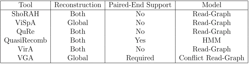
Table 1.2 Quasispecies reconstruction/inference tools and supported features.
All main tools currently support both local and global reconstruction.
All tools with the exception of QuasiRecomb utilize some form of a
LIST OF FIGURES
Figure 2.1 The case of two distinct reads for both amplicons . . . 13
Figure 2.2 Adding forks to the original s−t connected read graph. . . 17
Figure 2.3 Sensitivity results on simulated HCV population over error-free data.
The results are partitioned over each population distrubtion. . . . 21
Figure 2.4 Positive predictive value results on simulated HCV population over
error-free data. The results are partitioned over each population
dis-trubtion. . . 21
Figure 2.5 Jensen-Shannon divergence results on simulated HCV population over
error-free data. The results are partitioned over each population
dis-trubtion. . . 22
Figure 2.6 Sensitivity results on simulated HCV population over error-free data
for flow-based algoirthms. The results are partitioned over each
pop-ulation distrubtion. . . 25
Figure 2.7 Positive predictive value results on simulated HCV population over
error-free data for flow-based algoirthms. The results are partitioned
over each population distrubtion. . . 26
Figure 2.8 Jensen-Shannon divergence results on simulated HCV population over
error-free data for flow-based algoirthms. The results are partitioned
over each population distrubtion. . . 26
Figure 3.1 Results obtained from simulated amplicon reads HCV data using
sen-sitivity (weighted portion of true variants found). We relax the case
Figure 3.2 Results obtained from simulated shotgun reads HCV data using
sensi-tivity (weighted portion of true variants found). We relax the case of
requiring an exact match and allow for hamming distance. . . 34
Figure 4.1 Overview of high-fidelity sequencing protocol. (a) DNA material from
a viral population is cleaved into sequence fragments using any suitable
restriction enzyme. (b) Individual barcode sequences are attached to
the fragments. Each tagged fragment is amplified by the polymerase
chain reaction (PCR). (c) Amplified fragments are then sequenced. (d)
Reads are grouped according to the fragment of origin based on their
individual barcode sequence. An error-correction protocol is applied
for every read group, correcting the sequencing errors inside the group
and producing corrected consensus reads. (e) Error-corrected reads
are mapped to the population consensus. (f) SNVs are detected and
assembled into individual viral genomes. The ordinary protocol lacks
Figure 4.2 Overview of VGA. (a) The algorithm takes as input paired-end reads
that have been mapped to the population consensus. (b) The first step
in the assembly is to determine pairs of conflicting reads that share
dif-ferent SNVs in the overlapping region. Pairs of conflicting reads are
connected in the “conflict graph”. Each read has a node in the graph,
and an edge is placed between each pair of conflicting reads. (c) The
graph is colored into a minimal set of colors to distinguish between
genome variants in the population. Colors of the graph correspond
to independent sets of non-conflicting reads that are assembled into
genome variants. In this example, the conflict graph can be
mini-mally colored with four colors (red, green, violet and turquoise), each
representing individual viral genomes. (d) Reads of the same color
are then assembled into individual viral genomes. Only fully-covered
viral genomes are reported. (e) Reads are assigned to assembled
vi-ral genomes. Read may be shared across two or more vivi-ral genomes.
VGA infers relative abundances of viral genomes using the
expectation-maximization algorithm. (f) Long conserved regions are detected and
phased based on expression profiles. In this example turquoise and red
viral genome share a long conserved region(colored in black). There
is no direct evidence how the viral sub-genomes across the conserved
region should be connected. In this example 4 possible phasing are
valid. VGA use the expression information of every sub-genome to
resolve ambiguous phasing. . . 51
Figure 4.3 Genomic architecture of 44 real HCV viral genomes from 1739-bp long
fragment of E1E2 region. Length of longest common region shared
Figure 4.4 Accuracy of population size prediction. Up to 200 viral genomes were
generated from the Gag/Pol 3.4 Kb HIV region. The population
diver-sity is 5% - 10%. Variant abundances follow uniform (A) and
power-law (B). Highly-accurate 100x2 bp paired-end reads were simulated
from HIV population. . . 52
Figure 4.5 Assembly accuracy estimation. Up to 200 viral genomes were
gener-ated from the Gag/Pol 3.4 Kb HIV region. The population diversity is
3% - 20%. Variant abundances follow uniform (A) and power-law (B).
Consensus error-corrected 2x100bp paired-end reads were simulated
from HIV population. . . 52
Figure 4.6 Assembly accuracy estimation. Consensus error-corrected paired-end
reads of various lengths were simulated from a mixture of 10 real viral
clones from 1.3kb-long HIV-1 region. Assembly accuracy as measured
by sensitivity(A) and precision(B). Results are for 50,000 reads, no
improvement was observed when increasing the of number of reads. 53
Figure 4.7 Assembly accuracy estimation. Up to 200 recombinant viral genomes
were generated from the from 1.3kb-long HIV-1 region. Variant
abundances follow power-law and uniform. Consensus error-corrected
LIST OF ABBREVIATIONS
• NGS - Next Generation Sequencing
• MLE - Maximum Likelihood Estimate
• MAP - Maximum A-Posteriori
PART 1
INTRODUCTION
1.1 RNA Viruses and Viral Quasispecies
RNA viruses, as the name implies, encode their genome in RNA rather than DNA.
Notable examples include human immunodeficiency virus (HIV), hepatitis C (HCV), and
in-fluenza. RNA viruses display exceptionally high mutation rates in comparison to DNA-based
counterparts. Indeed, mutation rates varying between 10−4 and 10−6 per nucleotide have
been observed. In both experimental and natural infections, a viral particle, or virion, upon
infecting a cell may produce hundreds to thousands of progeny; thus, generating many
mu-tant strains into the population. In addition to mutations, RNA viruses have been known to
exhibit recombinant variants within the population. Cells can become co-infected by
differ-ent viral strains and consequdiffer-ently “cross over” genomes during replication. This process may
be repeated with the newly produced recombinant variants, further driving the heterogeneity
of the population. This population of closely related strains is known as a quasispecies.
The replicative dynamics ensure the virus can efficiently adapt to environmental changes
within an infected host. This mutational robustness is the root cause of difficulty for
ther-apeutic treatments. Therefore, accurately determining the viral population structure (i.e.,
individual genomes) is of great utility for both treatment and understanding of viral
quasis-pecies.
1.2 Sequencing Technologies
As a result of the rapid decrease in sequencing cost, it is now possible to directly
inspect a viral population. This massive amount of sequence data is generated using two
different processes. The first process is shotgun sequencing, whereby long genomic regions
Table 1.1 Next-generation sequencers and properties of the produced reads[1].
Manufacturer Avg Read Length Avg Read Count Avg Error Rate Paired/Mate Reads
Roche/454 450bp 1M 1.0% Yes (with kit)
Ion Torrent 200bp 60M 2.8% Yes
Illumina 150bp 10 1.0% Yes
Pacific Bio 8500bp 45k 12.0% No
amplicon sequencing, which is based on PCR amplification of a set of overlapping genomic
regions using sequence-specific primers. Multiple regions may be sequenced in a single run by
coupling the sequence-specific primers with “tags” or unique identification sequences. Table
1.1 gives a breakdown of various companies’ products and their respective specifications.
1.3 Viral Quasispecies Reconstruction Problem and Challenges
Due to the limitations of current sequencing technologies, entire viral genomes describing
a viral population cannot be accurately generated. Next-generation sequencers are capable of
produces massive amounts of genomic information, but are limited to short reads; therefore,
these genome snippits must be assembled.
Quasispecies Spectrum Reconstruction (QSR) Problem. Given a collection of
(shot-gun or amplicon) next-generation sequencing reads generated from a viral sample, reconstruct
the quasispecies spectrum, i.e., the set of sequences and the relative frequency of each sequence
in the sample population.
This task is challenging for the following reasons: (i) differentiating rare variants from
random sequencing errors and correcting systematic errors; (ii) deciding if multiple reads
with a concordant overlap belong to the same variant; (iii) and designing scalable software
to handle ever-increasing volumes of read-data.
1.4 Previous work
The first publicly available tool for reconstructing a viral quasispecies was ShoRAH [2].
[4]. Once the putative variants have been assembled, their relative abundances are computed
using an Expectation-Maximization (EM) algorithm. While ShoRAH manages to
success-fully capture the underlying population, it tends to vastly overestimate the true number of
variants, thus skewing accuracy. ShoRAH is available as a python program that can be run
for various forms a sequencing data: NGS shotgun data or single amplicon data.
The Viral Spectrum Assembler, or ViSpA[5], is another tool that reconstructs a
qua-sispecies by constructing a weighted read-overlap graph. The edge-weights in the graph
represent the probability of the overlap occurring between two sequencing reads. In order to
reduce the number of edges in the graph, a transitive closure is computed. This technique
removes “sub-reads” that add no further information to the population structure. ViSpA
repeatedly finds maximum-weight (i.e., high-probability) paths to cover the reads until the
graph is saturated. Similarly to ShoRAH, ViSpA utilizes an EM algorithm for estimating
variant frequencies. ViSpA is available as a java-based tool. While it was designed for NGS
shotgun data, in theory it could be applied to amplicon-based data as well.
QuRe [6] is a tool to reconstruct a viral quasispecies based on earlier work described in
[7]. Initially, the software aligns reads to a reference sequence, which are then corrected via
a Poisson process as described in [8]. Afterwards, reads are partitioned into sliding windows
using a randomized approach. Putative partitions are scored based on coverage, overlapping
sequence divergence, and internal window sequence divergence. A read-overlap graph is then
constructed, and paths are found by a hueristic. Once enough paths have been found, the
final results are then clustered based on error-rate parameters. QuRe is implemented in java
and runs on a variety of platforms.
QuasiRecomb is a software that employs a generative model to estimate the underlying
viral population[9]. It explicitly incorporates recombination into the model by utilizing
“generator” sequences. Each generator sequence is modeled by a hidden Markov model.
Recombination hotspots may occurr by “jumping” from one model to another at any given
point in the sequence space. The parameters to the model are estimated using an EM
Table 1.2 Quasispecies reconstruction/inference tools and supported features. All main tools currently support both local and global reconstruction. All tools with the exception of QuasiRecomb utilize some form of a read-graph.
Tool Reconstruction Paired-End Support Model
ShoRAH Both No Read-Graph
ViSpA Global No Read-Graph
QuRe Both No Read-Graph
QuasiRecomb Both Yes HMM
VirA Both No Read-Graph
VGA Global Required Conflict Read-Graph
estimate the population and respective abundances. QuasiRecomb is implemented in java
and targets single-amplicon data.
1.5 Contributions
We present novel “fork-resolution” algorithms for viral quasispecies reconstruction as
well as “flow”-based algorithms. Fork-resolution algorithms focus on solving local assembly
problems within the read-graph model. They are typically quite fast in practice, but are
limited in their accuracy. This inherent problem is a result of focusing only on small, local
assemblies. Flow-based algorithms take a more global approach to assembling the viral
population. After the read graph has been constructed, paths are found via network flows.
We have previously published work utilizing single-path network flows in addition to
multi-commodity flows. These algorithms and respective data-structures are implemented in a
Python framework called BIOA. The software is open source and is available for free.
Additionally, parameter estimation and model selection were contributed to the tool
kGEM. This software performs local reconstruction (short targeted region) of a viral
popu-lation and can be used for error correction. In order forkGEM to perform certain clustering,
a feasible error threshold must be determined. This is done using a simple p-value analysis
under Bonferonni adjustment. Finally, model selection is evaluated under both Akaike and
Bayesian information criteria.
our software Viral Assembler, or VirA. VirA first aligns the data using the InDelFixer
alignment tool and the random algorithm of QuRe to find good “virtual” amplicons over
NGS data. Once the partitions have been found,kGEM then locally reconstructs haplotypes
by correcting errors. Finally a read-graph is built over the local haplotypes and one of the
flow-based algorithms is run. VirA is implemented in Python, Java, and Scala. It runs on
multiple platforms and scales well as the number of reads grows.
1.6 Paper Roadmap
The paper is organized as follows. Chapter 2 discusses the model, methods, experiment
setup, and results for viral population reconstruction from error-free amplicon reads.
Fork-resolution methods are first described followed by the flow-based counterparts. Chapter 3
describes how to handle sequencing errors by thekGEM method. Our software VirA is then
described along with experiment setup and results. Chapter 4 presents the work completed
on paired-end data. Finally the paper outlines ongoing and future work in section 5.
1.7 Publications
Book Chapters
1. I. Astrovskaya, N. Mancuso, B. Tork, S. Mangul, A. Artyomenko, P. Skums, L.
Ganova-Raeva, I. M˘andoiu, and A. Zelikovsky “Inferring Viral Quasispecies Spectra
from Shotgun and Amplicon 454 Pyrosequencing Reads” Genome Analysis: Current
Procedures and Applications, 2013.
Journal Papers
1. Alexander Artyomenko, Nicholas Mancuso, Pavel Skums, Ion Mandoiu, Alex
Ze-likovsky, and Yury Khudyakov. “An EM-based Algorithm for Reconstructing a Viral
2. Pavel Skums, Nicholas Mancuso, Alexander Artyomenko, Bassam Tork, Ion
M˘andoiu, Yury Khudyakov, and Alex Zelikovsky. “Reconstruction of Viral
Popula-tion Structure from Next-GeneraPopula-tion Sequencing Data Using Multicommodity Flows”,
BMC Bioinformatics 2013, 14(Suppl 9):S2
3. Nicholas Mancuso, Bassam Tork, Pavel Skums, Lilia Ganova-Raeva, Ion M˘andoiu,
and Alex Zelikovsky, “Reconstructing Viral Quasispecies from NGS Amplicon Reads”
In Silico Biology, An International Journal on Computational Molecular Biology,
Vol-ume 11, 5. pp 237-249. 2012.
Conference / Workshop Papers
1. Serghei Mangul, Nicholas Wu, Nicholas Mancuso, Alex Zelikovsky, Ren Sun, and
Eleazar Eskin, “Accurate HIV population assembly from ultra-deep sequencing data”.
ISMB 2014.
2. Alexander Artyomenko, Nicholas Mancuso, Pavel Skums, Ion M˘andoiu, Alex
Ze-likovsky. “kGEM: An Expectation Maximization Error Correction Algorithm for Next
Generation Sequencing of Amplicon-based Data”, 9th International Symposium on
Bioinformatics Research and Applications. (Short Abstract), 2013.
3. Nicholas Mancuso, Bassam Tork, Pavel Skums, Ion M˘andoiu and Alex Zelikovsky
“Multi-Commodity Flow Methods for Quasispecies Spectrum Reconstruction Given
Amplicon Reads”, 8th International Symposium on Bioinformatics Research and
Ap-plications (Short Abstract), 2012.
4. N. Mancuso, B. Tork, P. Skums, L. Ganova-Raeva, I.I. M˘andoiu, A. Zelikovsky
“Workshop: A Maximum Likelihood Method for Quasispecies Spectrum Assembly”
Proc. 2nd Workshop on Computational Advances for Next Generation Sequencing
(CANGS 2012)
Beyah. “EDR2: A Sink Failure Resilient Approach for WSNs.” IEEE International
Conference on Communications (ICC), pp. 616-621, 2012.
6. N. Mancuso, B. Tork, I.I. M˘andoiu and A. Zelikovsky and P. Skums “Viral
Quasis-pecies Reconstruction from Amplicon 454 Pyrosequencing Reads”, Proc. 1st Workshop
on Computational Advances in Molecular Epidemiology, pp. 94-101, 2011
Posters
1. Serghei Mangul, Nicholas Wu,Nicholas Mancuso, Alex Zelikovsky, Ren Sun, Eleazar
Eskin, “Inferring HIV Quasispecies from Paired-End Reads”. RECOMB, April 2013.
2. Nicholas Mancuso, Bassam Tork, Pavel Skums, Ion M˘andoiu and Alex
Ze-likovsky, “Poster: Quasispecies Spectrum Reconstruction using Multi-commodity
Flows” RECOMB-Seq, April 2012.
3. S. Mangul, A. Caciula, N. Mancuso, I. M˘andoiu and A. Zelikovsky, “An Integer
Programming Approach to Novel Transcript Reconstruction from Paired-End RNA-Seq
Reads”, Poster at 16th Annual International Conference on Research in Computational
PART 2
METHODS FOR QUASISPECIES RECONSTRUCTION FROM AMPLICON
READS
2.1 Introduction and Contributions
In this section I present the amplicon (overlapping window) model for quasispecies
reconstruction. This model is selected for its simplicity and ease of analysis. Surprisingly
this model is still NP-hard to compute optimal solutions for (which we prove). Along with
the analysis, algorithms for reconstruction are proposed. These are divided along local
“fork-resolution” methods and slightly more global “flow”-based methods. All algorithms
are compared and validated against simulated hepatitis C (HCV) data. In addition to
reconstruction algorithms, a “graph-balancing” algorithm is presented. This method makes
a minimal amount of changes to the graph in order for all read-counts to be balanced. This
method vastly improves the local fork resolution methods, but seems to have little affect
on flow methods. However, this could be investigated further under more realistic read
generation scenarios.
2.2 Model
2.2.1 Likelihood and Entropy Minimization
The amplicon-based quasispecies assembly covers the full virus genome with the set
of K overlapping segments with predefined positions within the genome, called amplicons.
Each amplicon A1, . . . , AK has a predefined length and is sequenced to the same depth D,
i.e., covered with D reads. We distinguish two error models.
• The error-free model assumes that all reads are typing error-free or, equivalently, have
• The error-prone model allows some typing errors and additionally these errors should
be detected and fixed.
We also distinguish two frequency models.
• The ideal-frequency model assumes that in each amplicon’s distribution of reads is
identical and equal to the true distribution of quasispecies.
• The more realistic skewed-frequency model assumes that in each amplicon the
quasis-pecies are represented differently from the true distribution.
In the next subsection we address the QSR problem in the ideal-frequency model and then
show we can adjust frequencies to reduce the skewed-frequency model to the ideal-frequency
model.
The main goal is to reconstruct the genome-length quasispecies from amplicon data
consisting of K ×D reads. The secondary goal is to optimize the amplicon-based assembly
parameters K, D and amplicon positions in order to maximize the quality (sensitivity and
specificity) of assembly. We also compare the amplicon-based and the shotgun sequencing
approaches to quasispecies assembly. It is important to note that shotgun sequencing is more
prone to typing errors but less prone to frequency skewing than amplicon based sequencing.
Moreover, the methods for reconstruction of quasispecies from shotgun reads (e.g., ViSpA)
heavily rely on the uniform distribution. This allows a more accurate estimate of the
proba-bility of two overlapping reads coming from the same quasispecies. For reconstruction from
amplicon reads, this information is not available and therefore it is necessary to rely on
parsimonious considerations. Further, we discuss several related optimization formulations.
The following formulation is standard, but difficult to solve.
Most Parsimonious Spectrum. The most parsimonious spectrum requires the minimum
num-ber of distinct quasispecies that explains the observed reads. This formulation isNP-hard by
simple reduction from SUBSET SUM, which is defined as: given a (multi) set S of integers
Claim 1. QSR Problem is NP-hard.
Proof. Given an instance ofSUBSET SUM,S ={x1, . . . , xk}and countcwherePki=1xi =n,
letA1 ={r1, . . . , rk} be reads with counts{x1, . . . , xk} and A2 ={rk+1, rk+2}be reads with
counts {c, n−c}such that the overlap is consistent between any two reads ri ∈A1, rj ∈A2.
A minimal solution to the QSR problem will cover exactly k reads in A1. Taking the q≤k
reads and respective counts fromA1 that correspond to quasispecies containing readrk+1 we
find the solution to SUBSET SUM. If any read ri,0≤i≤k is split between rk+1, rk+2 there
must exist at least k+ 1 quasispecies (if all reads are covered) and will not be a minimal
solution.
However, a small number of different reads is expected within the same amplicon (small
number of quasispecies), allowing us to solve it exactly in practical time. The sets of
overlap-ping (adjacent) amplicons are partitioned into subsets with the same parts in the intersection
of these amplicons. The number of distinct reads in the overlap is at most the minimum of
the number of reads in the left and the right amplicons. Further, we discuss several models
and corresponding optimization formulations.
2.2.2 Quasispecies Assembly in the Error-Free, Ideal-Frequency Model Problem
The input data can be viewed as a K-staged read graph G = (V =V1 ∪ · · · ∪VK, E),
where
• each vertexvinVicorresponds to a distinct read in thei-th ampliconAiand has a count
c(v) (i.e., unique read v is repeated in the read sample c(v) times) P
v∈Vic(v) = D.
• each edge (u, v) connects two reads from consecutive amplicons Ai and Ai+1 which
agree in the overlap region
The solution can be viewed as the set Q = {qj} of u−v-paths, u ∈V1, v ∈ VK, each with
the frequency fj such that for each vertex v ∈V,
X
v∈qj
Given K amplicons A1, . . . , AK sequenced to the depth D, we need to assemble the
most likely full-length quasispecies and find their frequency distribution.
Rather than solving the K-staged assembly problem, we first focus on the two-staged
case, the solution to which is then used to “stitch” together all K stages. We therefore,
assume that there are only two stages, V1 and V2, thus implying that the read graph is
bipartite. A natural question is whether a feasible solution exists for this problem.
The problem can be reduced to consistency of linear equations. Letfebe the frequency
of the quasispecies e corresponding to the edge e = (u, v). Then for each vertex we write
the following constraint (2.1) to obtain the following system of linear equations:
∀v ∈V1∪V2
X
eincident tov
fe =c(v) (2.2)
The system of equations (2.2) is consistent if and only if the corresponding two-stage
assembly problem is feasible. Denote by G(c) the bipartite graph obtained from G by
splitting each vertex v into c(v) copies. It is clear that the following claim is true.
Claim 2. The system (2.2) is consistent if and only if G(c) has a perfect matching.
The feasibility of the two-stage assembly problem could be checked using any classical
perfect matching algorithm. We assume that (2.2) is consistent.
Theorem 1. Any solution of (2.2) with the minimal number of edges is a spanning forest
of G.
Proof. We assume thatGis connected. (2.2) could be written asIf =corI1f1+· · ·+Imfm =
c, whereI is the incidence matrix of G, Ij is the jth column of I.
Since Gis bipartite, rank(I) = n−1 [11]. Let the first n−1 columns and rows of I be
the basis columns and rows. The columns of the incidence matrix corresponding to the even
cycle are linearly dependent. Since G does not contain odd cycles, the edges e1, . . . , en−1
contain no cycles, and therefore form the spanning tree of G. Set free variables fn, . . . , fm
I0f0 =c0, (2.3)
where I0 is the sub-matrix of I restricted to the first n−1 columns and rows, f0 =
(f1, . . . , fn−1), c0 = (c1, . . . , cn−1).
As (2.2) is consistent, (2.3) is also consistent. Moreover, sinceGis bipartite,I is totally
unimodular [11]. This impliesI0 is also totally unimodular with rank(I0) = n−1. Therefore
(2.3) has a positive integer solution. The non-zero edges of this solution form the spanning
forest ofG.
This proves that (2.2) has a spanning forest solution. Letf be a solution of (2.2)
con-taining cycles. Consider a connected component of f, which has cycles. Find the acyclic
solution of (2.2) restricted to that component. This solution has a lesser number of edges.
Repeating this process for all connected components with cycles, we obtain the acyclic
solu-tion for (2.2).
Theorem 2. If there is a bipartite cycle between consecutive amplicons, then there is a
4-gamete rule violation, i.e., there should exist an additional (to existing in amplicons)
re-combination.
Proof. Let B be bi-cycle (a bipartite cycle) with 2k vertices (with k vertices in the left
amplicon Land with k vertices in the right amplicon R). For the sake of simplicity, assume
that the alphabet has two characters. Thenk different haplotypes inLcan be distinguished
in k −1 positions (the same for R). There are exactly 2k different edges in B. Assuming
no 4-gamete rule violation, we obtain 2k haplotypes distinguished in 2k−2 positions. This
implies a contradiction.
A simple maximum likelihood approach assumes that any edge (i.e., quasispecies) is
equally probable. As a result, it assigns non-zero frequencies to all possible quasispecies. A
more meaningful parsimonious approach requires that most likely solutions should contain
B b A a D d C c d≤b≤a≤c
Read A counta=c(A)
Read B countb=c(B)
Read C countc=c(C)
Read D countd=c(D)
AmpliconA1
Amplicon A2
[image:31.612.111.505.72.204.2]Common Overlap 6 = 6 = = = =
Figure 2.1 The case of two distinct reads for both amplicons
Let us make the case of two distinct reads for both amplicons. Assume that |V1| =
|V2| = 2, A and B are distinct reads in the first amplicon and C and D are in the second
(see Fig. 2.1). Furthermore, let all four possible combinations of reads be consistent in their
overlap.
On the left there are four reads and on the right there is the corresponding graph.
Without loss of generality, assume that d ≤ b ≤ a ≤ c. If a = c, then b = d and we can
have the minimum possible number of two non-zero edge frequencies. If a6=c, then the four
constraints have rank three and there should be three edges with non-zero frequency. There
are two possibilities for three non-zero frequency edges:
• AC =a, AD= 0, BC =c−a,and BD=d
• AC =a−d, AD=d, BC =b,and BD= 0
The first case is more probable if a > b and is equally probable if a = b. A simple
maximum likelihood does not appear to be an efficient approach given these assumptions.
We now formalize a more sophisticated model to compute maximum likelihood. We define
a “fork”F = (L, R) to be a bi-clique with partitionsLand R, where |L|=l,|R|=r. Given
a model, we would like to be able to compute the probability of observing the reads in L
and R. As reads in both partitions overlap, no single instance of a quasispecies is capable of
producing both its read inLand its read inR. Based on this reasoning, we assume that the
For simplicity we may assume that each quasispecies containing overlap ofF produces
exactly one read. In other words, if a quasispecies does not “emit” a read then we
con-sider it nonexistent. Any possible resolution of XF of the fork F consists of c(L) +c(R)
instances formed by lrdistinct quasispeciesq11, . . . , qlr with countsx11, . . . , xlr. We consider
a resolution XF to be feasible ifXF ={xij} wherexij =xLij +xRij such that
r
X
j
xLij =ci, ∀i∈L (2.4)
l
X
i
xRij =di, ∀j ∈R.
Following the model (eq. 2.4) we estimate the probability P(XF) that XF produces the
observed reads L and R as follows. We can see there are in total TF = 2c(L)+c(R) ways
to produce reads from c(L) +c(R) quasispecies restricted to two amplicons. We need to
count the number of ways to produce the observed read counts, C(XF), in order to find
P(XF) = C(TXF)
F .
We make one more assumption that the resolution XF is a forest (see theorem 1). For
a given leaf i and count ci we can see that there exists a single quasispecies qij with count
xij ≥ ci that is capable of emitting all copies of the i-th read. The number of possible
assignments of quasispecies to produce this read is xij
ci
. Let F0 be the fork obtained from
F by removing quasispecies qij and decreasing the count of the stem j-th read by xij −ci.
We now have,
C(XF) =C(XF0)·
xij
xL ij
(2.5)
=C(XF0)·
xij!
The formula (2.5) defines the recursive computation of the likelihood given a forest resolution
XF for the fork F = (L, R). The computation can be done in leaf-removal order i.e.,
v1, . . . , vl+r−k, where k = k(XF) is the number of connected components of XF. Let the
remaining count of a leaf vi be ci, the count of the covering quasispecies qij be xij and the
count of the j-th stem’s read be cj. The definition is as follows,
L(XF|F = (L, R)) =P(XF) (2.6)
= C(XF)
TF
(2.7)
=
Ql+r−k i=1
xi
ci
2c(L)+c(R) . (2.8)
Therefore, maximizing the log-likelihood is equivalent to maximizing,
logC(XF) = l+r−k
X i=1 log xi ci .
Following [12], we notice that maximizing likelihood is equivalent to minimizing Shannon
Entropy, which is defined as follows,
−
n
X
i=1
p(xi) logp(xi).
The more quasispecies we have, the higher the entropy value. Therefore, finding a
solu-tion with the minimum amount of quasispecies reduces the entropy of the solusolu-tion, which
corresponds to the idea of a most parsimonious solution.
Minimum Entropy Quasispecies Assembly Problem. Given a read graph with
fre-quencies on reads, find the set of quasispecies (paths) and respective frefre-quencies that explains
all reads and frequencies, such that the resulting set has minimum entropy.
The read graph for two amplicons consists of a set of disjoint bi-cliques, each
corre-sponding to a distinct overlap-part. The number of quasispecies cannot exceed the minimum
2.2.3 Reduction of Skewed-Frequency Model to Ideal-Frequency Model
We would like to reduce this problem to the case in which all frequencies of the reads are
ideal. First, we formulate the problem of balancing forks in the graph, which is equivalent
to estimating ideal frequencies of the reads. We then suggest two approaches.
A fork f = (L, R), where L and R are the sets of reads from the left and the right
amplicons, respectively, is balanced if the total frequencies ofLandRare equal to each other.
It is obvious that any ideal-frequency amplicon-read spectrum has all its forks balanced. The
opposite is also true, i.e., any amplicon-read spectrum with balanced forks has a feasible
quasispecies spectrum which has ideal frequencies.
Fork Balancing Problem. Given a spectrum of amplicon reads R = {ri} with observed
frequencies O = {oi} and forks fj = (Lf, Rf) find ideal frequencies F = {fi} such that all
forks are balanced.
Least Squares Approach via Quadratic Program. We model the fork balancing
prob-lem as a quadratic program (QP) with linear constraints (equation 2.9). The approach looks
for the minimum squared adjustment of observed read frequencies, X ={xi}. We can
gen-eralize this method by allowing weights to be used in the objective. The justification for
allowing weights is to normalize adjustment values. We expect that a read with high
fre-quency may be adjusted to a greater extent than a read with a very small frefre-quency. Typical
weight values for reads are wi = c1i, whereci is the frequency of readi.
Minimize :Xwix2i (2.9)
Subject to: X
i∈Lf
(xi+oi) =
X
i∈Rf
(xi+oi), ∀f ∈ Forks (2.10)
xi +oi ≥0 (2.11)
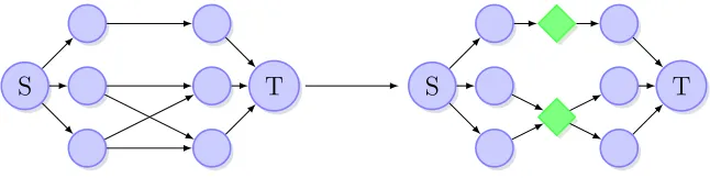
Graph Data Structure. Building aK-staged read graph fromK amplicons is
S T S T
Figure 2.2 Adding forks to the original s−t connected read graph.
Ai+1. If a consistent read exists, add both reads as vertices to the graph with a directed edge
joining them. Repeat this for K amplicons Ai, . . . , AK. Add a single source S connected
with all reads in the first amplicon and single sink T with edges from all reads in the last
amplicon.
Before the final structural modification is made in the graphG, we may wish to adjust
the frequencies. This may be done by either solving the QP (eq. 2.9) or by simple scaling.
To scale the frequencies of each complete bipartite subgraph in the directed graphG, find the
sum of the frequencies in the first and second partitions. If they do not equal one another,
scale the values in the right partition to frequencies in the left. This may be completed for
the entire graph in a breadth first manner from the source to the sink.
The graph will be composed of bipartite cliques (bi-clique), with each clique representing
a consistent overlap in the reads. The graph is then transformed by adding a fork vertex
for each bi-clique. Given a bi-clique Kn,m, add an edge fromn vertices in the first partition
to the fork vertex and an edge from the fork vertex to the m in the second partition. This
modification reduces the amount of n ·m edges from each original bi-clique to a “forked”
subgraph with n+m edges. This is repeated for all bi-cliques in the graph (figure 2.2).
2.3 Experiment Setup and Validation Metrics
2.3.1 Datasets and Experiment Design
In order to perform cross-validation on the assembly method, we simulate reads data
frequencies are generated according to some specific distribution. In our simulation
experi-ments, we use a uniform, geometric, and skewed distribution to create sample quasispecies
populations with different number of randomly selected above-mentioned quasispecies
se-quences. Reads are simulated without sequencing errors. The length of a read follows a
normal distribution with mean value of 320bp and variance 10bp. The starting position
follows a uniform distribution. The total amount of reads varies from 5K, 20K, to 100K.
2.3.2 Validation Metrics
Sensitivity is defined as |T rueP ositives|T rueP ositives|+|F alseN egatives| | and is a measure of a test’s positive
identifications. We utilize this metric as a measure of the quality assembled quasispecies.
If a candidate quasispecies has an exact match (in terms of its sequence) in the simulated
quasispecies, we consider it a true positive match. Thus sensitivity is a function of the
number of correctly assembled quasispecies out of the population. Positive predicted value
(PPV) is the ratio of correctly identified quasispecies over assembled quasispecies. It is
defined as |T rueP ositives|T rueP ositives|+|F alseP ositives| |. It is useful for cross-validating a given method, by
highlighting the amount of incorrectly assembled quasispecies.
Jensen-Shannon divergence is a quasi-metric that measures the divergence (i.e.,
dis-tance) between two statistical distributions. It differs from the Kullback-Leibler divergence
due to the addition of a midpoint. This allows for the quasi-metric to be continuous over
all values of P and Q. As the size of our reconstructed spectrum may differ from the size of
the “true” spectrum, we can still gain insight into how close the two are. It is defined as:
JSD(P||Q) = 1
2DKL(P||M) + 1
2DKL(Q||M)
where
DKL(P||Q) = n
X
i=1
P(i) logP(i)
Q(i)
and M = 12(P +Q). By taking as assembled quasispecies spectrum and computing the
frequency distribution is to the true spectrum.
2.4 Local Fork Resolution-based Methods for Reconstruction
2.4.1 Greedy Algorithm for Fork Resolution
Each fork vertex v (a vertex with at least two in-edges and two out-edges) should be
resolved, i.e., a resolution (acyclic graph connecting inputs with outputs) should replace v.
We greedily resolve forks in the graph by placing left and right vertices into priority queues
L and R. Extract the maximum from L and from R and create a new edge (maxl, maxr).
The frequency of the new edge is min(maxl, maxr). Decrease the key (frequency) of both
vertices and reinsert the larger maximum frequency; otherwise, both vertices are exhausted
and no longer considered for further resolution. When either L or R are empty, the round
is completed, and the fork vertex is removed. This is done recursively until no forks are left
in the graph. It may be the case that read vertices (not just overlap vertices) become forks
after a round and are eligible for resolution.
2.4.2 Minimum Forest Fork Resolution
Rather than rely on a greedy heuristic, we also employed an integer linear program
(ILP) that minimizes absolute value difference of observed and assigned read counts, such
that all reads belong to a tree. The resulting solution will be a forest over a bi-clique. Given
is given as,
Minimize: X
i∈L
yi
Subject to:
L
X
i
xij = 1 ∀j ∈R
R
X
j
rj·xij −li ≤yi ∀i∈L
li− R
X
j
rj ·xij ≤yi ∀i∈L.
The intuition is that leaves in the forest assign “all” their reads to a single parent. Internal
nodes “balance” out the counts of its children counts. The optimal solution will be the forest
that is most balanced in terms of assigned reads.
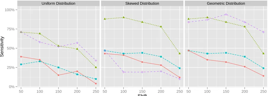
2.5 Results
Experiment results clearly indicate the ability of the greedy fork-resolution algorithm to
reconstruction the population accurately, as shown in figures (2.3-2.5). This is particularly,
noticeably under the skewed and geometric distributed populations. Interestingly, results
for the minimum forest solution were much worse than the greedy, despite being an exact
solution to the ILP. This is most likely a result of the ILP minimizing total deviation, and not
directly minimizing entropy. However, both algorithms outperform the guide distribution
method (GD).
When validating the quality of assigned abundances, the greedy method performs
ex-ceedingly well given both skewed and geometric distributed populations. In fact, all methods
tend to perform much better on average under non-uniform distributions. Unlike the
uni-formly distributed population, as the abundances of variants under the skewed and geometric
● ● ● ● ● ● ● ● ● ● ● ● ● ● ●
Uniform Distribution Skewed Distribution Geometric Distribution
0% 25% 50% 75% 100%
50 100 150 200 250 50 100 150 200 250 50 100 150 200 250
Shift
Sensitivity
[image:39.612.79.531.143.306.2]Method ● Greedy Method Guide Distribution Minimum Forest
Figure 2.3 Sensitivity results on simulated HCV population over error-free data. The results are partitioned over each population distrubtion.
● ● ● ● ● ● ● ● ● ● ● ● ● ● ●
Uniform Distribution Skewed Distribution Geometric Distribution
0% 25% 50% 75% 100%
50 100 150 200 250 50 100 150 200 250 50 100 150 200 250
Shift
PPV
Method ● Greedy Method Guide Distribution Minimum Forest
[image:39.612.79.534.472.637.2]● ●
● ●
●
● ● ● ●
●
● ● ● ●
●
Uniform Distribution Skewed Distribution Geometric Distribution
25% 50% 75% 100%
50 100 150 200 250 50 100 150 200 250 50 100 150 200 250
Shift
JS Div
ergence
[image:40.612.80.533.109.272.2]Method ● Greedy Method Guide Distribution Minimum Forest
Figure 2.5 Jensen-Shannon divergence results on simulated HCV population over error-free data. The results are partitioned over each population distrubtion.
2.6 Flow-based Methods for Quasispecies Reconstruction from Amplicon Reads
2.6.1 Maximum-Bandwidth Algorithm
A maximum bandwidth path in a graph G is a path from a sourceS to a sink T, such
that the bandwidth corresponds to the minimum capacity (frequency) edge in the path.
One method to resolve the QSR problem is to continually find maximum bandwidth paths
through the read graph. Repeat the following until S and T are disconnected (cannot exist
an edge with frequency/count of zero or less than some number >0 for real valued edges):
Find an S −T max-bandwidth path P with bandwidth m. Subtract bandwidth m from
G-edges of P. This will exhaust at least one edge in the path, forcing the next iteration to
choose a new path. Frequencies of the quasispecies are normalized from a count (maximum
bandwidth) to a percentage simply by dividing a quasispecies count over the sum of all
2.6.2 Maximum Frequency Path
A maximum frequency path in a graphGis a path from a sourceSto a sinkT, such that
the total frequency of the path is maximized. If frequencies are integer values, a maximum
frequency path is equivalent to the longest path of the graph G. While LONGEST PATH
is NP-hard in the general case, it is solvable in polynomial time on acyclic graphs using
dynamic programming[10]. If the graph G is a directed acyclic graph (as is our case), it
may be solved in linear time by using a topological ordering of vertices combined with
dynamic programming for computing path lengths. Maximum frequency paths may be used
to resolve the QSR problem in a fashion similar to the maximum bandwidth path method. In
other words, until there exists no path from the source S to the sink T, find the maximum
frequency path P with total frequency f. Set the corresponding frequency in G to 0 for
each edge in the path P. Repeat until no non-zero frequency paths exist. Path frequencies
are then normalized in the same manner as maximum bandwidth path. The concept is
inspired by the greedy approximation algorithm for MIN ENTROPY SET COVER from [12].
The OP T + 3 approximation is achieved by greedily selecting a set that covers the most
elements from the universe. After removing the selection from the universe, the algorithm
repeats on the remaining sets until nothing is left to be covered. In a similar fashion, our
algorithm covers the largest possible amount of reads in the graph, removes them, and then
recurses.
2.6.3 Multi-commodity Flow Algorithm
While the previous flow-based algorithms utilize more global information then the local
fork-resolution methods, solutions are still found iteratively. This may result in non-optimal
solutions with respect to parsimony. This shortcoming can be addressed by modelling the
problem as a multi-commodity flow. Given parameterk, the optimal solution to the following
mixed integer program corresponds to k paths in the graph that cover all reads. The ILP is
Minimize: X
0≤i≤k
(s,u)∈E
fs,ui
Subject to:
k
X
i
gu,vi ≥cu,v ∀(u, v)∈E
X
u∈pred(v)
giu,v = X
u∈succ(v)
giv,u ∀v ∈V, i= 1. . . k
X
u∈succ(v)
fv,ui = 1 ∀v ∈V, i= 1. . . k
fu,vi ≥gv,ui ∀(u, v)∈E, i= 1. . . k
fu,vi ∈ {0,1} ∀(u, v)∈E, i= 1. . . k
gu,vi ∈[0,1] ∀(u, v)∈E, i= 1. . . k
where f variables represent the binary-flow over an edge, and g variables represent the
fractional amount of flow. Together, these variables indicate which edges to select and what
percentage of reads will be assigned to a given flow. Without the binary variable, it would
not be possible to constrain the fractional flow to single paths. A consequence of this is that
this ILP cannot be solved in polynomial time in the worst case. However, in practice it is
found to perform quite well.
2.6.4 Results
Maximum bandwidth outperforms the maximum frequency method as well as guide
distribution method in terms of sensitivity for quasispecies with uniform distribution (see
figure 2.6). It correctly assembles seven out of ten quasispecies on average over the data set
when given 100K reads and window length 300bp. As shift position increases (less overlap
between windows) the quality of all four methods degrades. A shorter overlap would
pro-duce bi-cliques of larger size in the subgraph, which increases the complexity of the problem.
● ● ● ● ● ● ● ● ● ● ● ● ● ● ●
Uniform Distribution Skewed Distribution Geometric Distribution
0% 25% 50% 75% 100%
50 100 150 200 250 50 100 150 200 250 50 100 150 200 250
Shift
Sensitivity
[image:43.612.79.532.108.271.2]Method ● Guide Distribution Max Bandwidth Max Frequency MinFlow
Figure 2.6 Sensitivity results on simulated HCV population over error-free data for flow-based algoirthms. The results are partitioned over each population distrubtion.
the multi-commodity method assemble between eight and nine out of ten correct variants of
the population, while GD and maximum frequency produce four out of ten (see figure 2.6).
Similarly under the geometric distribution, maximum bandwidth and the greedy resolution
method correctly produce approximately nine and eight out of ten respectively, with GD
and maximum frequency reconstructing five out of ten (see figure 2.6). Interestingly,
pos-itive predicted values for maximum frequency path tend to be more competpos-itive with the
other methods despite its typically lower sensitivity. This is most likely the result of
max-imum frequency paths quickly covering many reads in the graph each iteration (see figure
2.7). Similarly for maximum bandwidth, which exhausts the graph much faster than greedy
methods.
2.7 Extension to Shotgun Reads
So far, we have focused on solving the reconstruction problem given amplicon reads.
Still, shotgun sequencing offers a viable alternative approach. The benefit of shotgun
se-quencing is that it does not require complicated primer design of targeted regions. In order
● ● ● ● ● ● ● ● ● ● ● ● ● ● ●
Uniform Distribution Skewed Distribution Geometric Distribution
0% 25% 50% 75% 100%
50 100 150 200 250 50 100 150 200 250 50 100 150 200 250
Shift
PPV
[image:44.612.79.532.143.307.2]Method ● Guide Distribution Max Bandwidth Max Frequency MinFlow
Figure 2.7 Positive predictive value results on simulated HCV population over error-free data for flow-based algoirthms. The results are partitioned over each population distrubtion.
● ● ● ● ● ● ● ● ● ● ● ● ● ● ●
Uniform Distribution Skewed Distribution Geometric Distribution
25% 50% 75% 100%
50 100 150 200 250 50 100 150 200 250 50 100 150 200 250
Shift
JS Div
ergence
Method ● Guide Distribution Max Bandwidth Max Frequency MinFlow
[image:44.612.79.532.471.636.2]to the amplicon scenario. Indeed, by finding short overlapping window segments that span
the region we can proceed with any of the previously described algorithms.
Given a set of shotgun reads and parameters for minimum and maximum window size,
we reduce the shotgun quasispecies reconstruction problem to the amplicon case as follows.
First, calculate sequencing statistics such as positional coverage and entropy. By calculating
positional entropy, we have an idea on how diverse a given locus is. The rational is to
partition the reads in such a way to have highly diverse overlaps. This reduces the overall
complexity of the reconstruction problem. While there will be more forks, each fork will
fewer possible choices. Random search is applied to intervals over the region of interest
and scored based on Z-score statistics. This method was described initially in [14]. It runs
quickly and finds acceptable overlaps rather than naively partitioning based on some fixed
PART 3
CORRECTING SEQUENCING ERRORS IN QUASISPECIES
RECONSTRUCTION
3.1 Introduction and Contributions
In this section I present a formal derivation of the E and M steps for an EM algorithm
to compute the maximum likelihood estimates for our generative model. This includes the
mixture weights (i.e., genotype frequencies) along with the sequencing error-rates for each
sequenced position. Prior to this, kGEM had not been fully formalized with some steps
still needing justification. Additionally, this derivation elucidates the flexibility of the EM
algorithm and how to estimate model parameters beyond simple mixing weights.
Furthermore, I describe software for reconstructing a viral population from NGS reads
(shotgun or amplicon) dubbed Viral Assembler (VirA). The software is a combination of
both Java and Python. It makes use of state-of-the-art alignment software InDelFixer along
with error-correction software kGEM. Once reads have been aligned, windows have been
found, and reads corrected, VirA builds a read-overlap graph and computes a path-packing
heuristic.
3.2 Error Correction by kGEM
The proposedkGEM algorithm attempts to find the set of variants (haplotypes) which
is the most likely producing the observed set of reads R. We first describe an alignment
of reads to the extended reference sequence and formally introduce the notion of a
popu-lation genotype (fractional haplotype). Next we describe the iterative procedure of kGEM
consisting of initialization and genotypes estimation.
The extended reference is obtained by identification of insertions using pairwise
of insertions. It may contain deletions due to insertions in reads, which we denote by the
symbol d. We prioritize gap-minimization over mismatches minimization since we need to
minimize the length of extended reference N. For each read, we assume that enumeration
of alleles in it is the same as in the extended reference.
The population P could be represented as frequency distribution of alleles at each
position of extended reference. Formally, given a population P, a genotype G = G(P) of
the population P is a matrix where each column corresponds to a position on the extended
reference and each row corresponds to the allele {a,c,t,g,d}. Each entry fm(e) is the
frequency of allelee in mth position of genotype G, P
efm(e) = 1.
The algorithm finds a set of genotypes {G1, G2, . . . , Gk} which most adequately
repre-sents the population P. We initialize this set by selecting reads covering entire sequence
space of the population P. In greedily manner we search for a read that maximizes the
minimum Hamming distance to previously selected reads.
We now describe the generative model that characterizes the production of reads from
genotypes. We define the probability that genotype Gi generated read r as
Pr[r|Gi] = |r|
Y
j=1
(1−4j)I[rj=Gij]I
[rj6=Gij]
j
where is the error-rate of the sequencing technology. The likelihood (and log-likelihood) of
the population genotypes G along with their respective frequencies f is given by,
L(G, f;R) = Y
r∈R k
X
i=1
fiPr[r|Gi]
!nr
(3.1)
`(G, f;R) =X
r∈R
nr·log k
X
i=1
fiPr[r|Gi]
!
(3.2)
(3.3)
where R is the set of distinct reads and nr is the multiplicity of read r. As this function is
log-likelihood defined as,
`c(G, f;R) =
X
r∈R k
X
i=1
nrI[zr =i] log(fiPr[r|Gi]) (3.4)
where I is the indicator function and zr are variables indicating which genotype generated
read r. However, as we cannot possibly know a-priori values for I[zr = i] we solve for the
expected complete-data log-likelihood
Q(G, Gt−1) =E "
X
r∈R k
X
i=1
nrI[zr =i] log(fiPr[r|Gi])
#
(3.5)
=X
r∈R k
X
i=1 nr
pri
z }| {
E[I[zr =i]] log(fiPr[r|Gi]) (3.6)
=X
r∈R k
X
i=1
nrprilog(fi) +
X
r∈R k
X
i=1
nrprilog(Pr[r|Gi]). (3.7)
The MLE parameters can be found by the EM algorithm. The E-step is computed by simple
Bayes’ theorem,
pri =
fiPr[r|Gti−1]
P
i0fi0Pr[r|Gt−1
i0 ]
. (3.8)
The M-step for genotype frequenciesf are computed by taking the derivative of Qwrt tof
with the added lagrange constraint that P
ifi = 1,
fi =
P
r∈Rnrpri
Genotype error-rates (with slightly more work) are computed by ∂Q ∂j = 4 Nj
z }| { X
r∈R k
X
i=1
nrpriI[rj =Gij])
4j −1
+ P
r∈R
Pk
i=1nrpri(1−I[rj =Gij])
j
(3.10)
= 4Nj 4j −1
+ |R| −Nj
j
(3.11)
j =
|R| −Nj
4|R| (3.12)
where Nj is the weighted number of matches in position j. We see that this calculation
also makes intuitives sense: the error rate is the proportion of weighted mismatches to (four
times) the number of reads. The reason four shows up is to account for an error being
possible for each of the 3 other nucleotides (or deletion).
3.2.1 Threshold Determining
Dispite being able to infer the error-rates for the sequenced population, it would still
be useful to filter results based on statistical significance. Hence, we utlize a simple test to
determine the minimum possible thresholdtj for a given position. If a given genotype does
not meet this criterion it is dropped from consideration. The EM algorithm estimates the
sequencing error-rate, hence we can find define the probability that there exist at least q
errors in position j as
fj(q) = Pr[Num errors in position j ≥q] =
X
θ=q
|R|
θ
θj(1−j)|R|−θ. (3.13)
We can determine the minimum thresholdtj given a Bonferroni corrected statistical
signifi-cance α/cby computing
tj = arg min t
(fj(t)≤α/c)
where cis the number of reads. As fj is a distribution function and therefore monotonic,tj
3.2.2 Model Selection
kGEM provides a reasonable model to correct errors in a small viral genomic region.
However, selecting k a-priori may be difficult. To address this issue, model selection may
be performed. We investigated both Akaike information criterion (AIC) and the Bayesian
information criterion (BIC). Given k (model size) and ` (log-likelihood), and n (number of
data points), AIC and BIC are defined as,
1. AIC = 2k−2`
2. BIC =klogn−2`.
A straightforward application to kGEM may seem at first a beneficial idea; however,
the “final” k is typically much less than the original k. This is a result of the algorithm’s
default behavior. Genotypes with frequency less than a given threshold are dropped while
others may be merged. To adjust for this, the threshold value can be set to 0.
3.3 VirA: Viral Assembler
VirA takes as input the read data in fasta format, a reference, and the
sequence-specific primers used for amplicon experiments. Reads are aligned to the reference using
InDelFixer version 0.8[15] and then partitioned into amplicons. The individual amplicons
are re-aligned to adjust for potential frame-shifts and corrected for sequencing errors using
the tool kGEM[16]. All corrected amplicons are recombined for a final alignment before
reconstruction. This reduces the possibility for frame-shift in overlapping segments. A
read-overlap graph is then constructed for assembly. Depending on the parameters, VirA
performs either the maximum bandwidth-path heuristic[17] or the exact algorithm based
on a multi-commodity flow formulation[18] to reconstruct the viral population. Briefly, the
maximum-bandwidth algorithm iteratively searches for the best possible single-path flow.
After a path is found the read-counts are updated and the algorithm tries again. This
con-tinues until the graph reaches saturation. The multi-commodity approach simultaneously
● ● ● ● ● ● ● ● ● ● ● ● ●● ● ● ●● ● ● ● ● ● ● Power−law Uniform 0% 25% 50% 75% 100%
0 1 2 3 4 5 0 1 2 3 4 5
Allowed Hamming Distance
Method ●
● QuRe
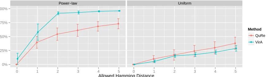
[image:51.612.90.527.78.204.2]VirA
Figure 3.1 Results obtained from simulated amplicon reads HCV data using sensitivity (weighted portion of true variants found). We relax the case of requiring an exact match and allow for hamming distance.
3.4 Datasets and Experiment Design
To validate VirA we simulated 10 viral populations from a sample of 43 HCV
vari-ants targeting the E1E2 region. Each population was duplicated into two data sets with
variant abundances adhering to a uniform and power-law (α = 2.0) distribution. Primers
were designed to generate between 7 to 12 amplicons covering the 1734nt long region for
amplicon-based reads. Both amplicon and shotgun-based reads were generated using Grinder
version 0.5 containing mutation errors (substitution & indel) uniformly at 0.1% along with
homopolymer errors according to the Balzer model[19]. Weighted sensitivity and positive
predictive value were used to assess the reconstructed population quality
3.5 Results
We validated VirA against QuRe using simulated HCV sequencing data. In all of the
cases VirA outperformed QuRe in both sensitivity and ppv. While results for both programs
are mediocre, this may be attributed to the aggressive error model used to simulate reads.
By only using a homopolymer error model rather than the additional mutational errors, we
●
● ●●
●
●
●
●
●
●
●
●
●
●
●
●
●
●
●
●
●
●
●
●
Power−law Uniform
0% 25% 50% 75% 100%
0 1 2 3 4 5 0 1 2 3 4 5
Allowed Edit Distance
Method
●
●
QuRe
[image:52.612.93.522.300.434.2]VirA
![Table 1.1 Next-generation sequencers and properties of the produced reads[1].](https://thumb-us.123doks.com/thumbv2/123dok_us/9140212.989109/20.612.73.559.94.170/table-generation-sequencers-properties-produced-reads.webp)