Using a multi hypothesis framework to improve the understanding of flow dynamics during flash floods

https://doi.org/10.5194/hess-22-5317-2018 © Author(s) 2018. This work is distributed under the Creative Commons Attribution 4.0 License.

Using a multi-hypothesis framework to improve the understanding

of flow dynamics during flash floods

Audrey Douinot1, Hélène Roux1, Pierre-André Garambois2, and Denis Dartus1

1_{Institut de Mécanique des Fluides de Toulouse (IMFT), University of Toulouse, CNRS – Toulouse, France}

2_{Laboratoire des Sciences de l’ingénieur, de l’informatique et de l’imagerie (ICUBE) – INSA Strasbourg, Strasbourg, France}

Correspondence:Audrey Douinot ([email protected]) Received: 4 December 2017 – Discussion started: 8 December 2017

Revised: 14 September 2018 – Accepted: 18 September 2018 – Published: 16 October 2018

Abstract. A method of multiple working hypotheses was applied to a range of catchments in the Mediterranean area to analyse different types of possible flow dynamics in soils during flash flood events. The distributed, process-oriented model, MARINE, was used to test several repre-sentations of subsurface flows, including flows at depth in fractured bedrock and flows through preferential pathways in macropores. Results showed the contrasting performances of the submitted models, revealing different hydrological be-haviours among the catchment set. The benchmark study of-fered a characterisation of the catchments’ reactivity through the description of the hydrograph formation. The quantifi-cation of the different flow processes (surface and intra-soil flows) was consistent with the scarce in situ observations, but it remains uncertain as a result of an equifinality issue. The spatial description of the simulated flows over the catch-ments, made available by the model, enabled the identifica-tion of counterbalancing effects between internal flow pro-cesses, including the compensation for the water transit time in the hillslopes and in the drainage network. New insights are finally proposed in the form of setting up strategic moni-toring and calibration constraints.

1 Introduction

1.1 Flash flood events: an issue for forecasters

Flash floods are “sudden floods with high peak discharges, produced by severe thunderstorms that are generally of lim-ited areal extent” (IAHS-UNESCO-WMO, 1974; Garam-bois, 2012; Braud et al., 2014). They are often linked to

localised and major forcings (greater than 100 mm; Gaume et al., 2009) at the heads of steep-sided, mesoscale catch-ments (with surface areas of 10–250 km2).

The large specific discharges and intensities of precipita-tion lead to the flash floods being classified as extreme. Nev-ertheless, those events are not scarce nor unusual, since on average, there were no fewer than five flash floods a year in the Mediterranean Arc between 1958 and 1994 (Jacq, 1994), and they tend to be amplified against a background of climate change (Llasat et al., 2014; Colmet Daage et al., 2016). Flash floods constitute a significant hazard and are therefore a con-siderable risk for populations (UNISDR, 2009; Llasat et al., 2014). They are particularly dangerous due to their charac-teristics, namely that (i) the suddenness of events makes it difficult to warn populations in time, and this can lead to panic, thus increasing the risk when a population is unpre-pared (Ruin et al., 2008), (ii) the traditional connected mon-itoring systems are not adapted to the temporal and spatial scales of the flash floods (Borga et al., 2008; Braud et al., 2014), and (iii) the magnitude of floods implies significant amounts of kinetic energy, which can transform transitory rivers into torrents, resulting in the transport of debris rang-ing from fine sediments to tree trunks as well as the scourrang-ing of river beds and the erosion of banks (Borga et al., 2014).

1.2 Flash flood events: understanding flow processes Due to the challenges involved in forecasting flash floods, there has been considerable research done on the subject over the last 10 years. Examples include the HYDRATE (Hy-drometeorological data resources and technologies for effec-tive flash flood forecasting, 2006–2010; Gaume and Borga, 2013), which enabled the setting up of a comprehensive Eu-ropean database of flash flood flash events as well as the de-velopment of a reference methodology for the observation of post-flood events, the EXTRAFLO (EXTreme RAinfall and FLOod estimation, 2009–2013; Lang et al., 2014) to estimate extreme precipitation and floods for French catchments, the HYMEX project (HYdrological cycle in the Mediterranean EXperiment, 2010–2020; Drobinski et al., 2014) focusing on the meteorological cycle at the Mediterranean scale and particularly on the conditions that allow extreme events to develop, the FLASH project (Flooded Locations and Simu-lated Hydrographs, 2012–2017; Gourley et al., 2017) assess-ing the ability and the improvement of a flash flood forecast-ing framework in USA on the basis of real-time hydrologi-cal modelling with high-resolution forcing, or the FLOOD-SCALE project (Multi-scale hydrometeorological observa-tion and modelling for flash floods understanding and sim-ulation, 2012–2016; Braud et al., 2014), based on a multi-scale experimental approach to improve the observation of the hydrological processes that lead to flash floods.

In the northwestern Mediterranean context – especially concerned with specific autumnal convective meteorologi-cal events – the European cited research particularly demon-strates the importance of cumulative rainfall (Arnaud et al., 1999; Sangati et al., 2009; Camarasa-Belmonte, 2016), the previous soil moisture state (Cassardo et al., 2002; Marchan-dise and Viel, 2009; Hegedüs et al., 2013; Mateo Lázaro et al., 2014; Raynaud et al., 2015) and the storage capac-ity of the area affected by the precipitation (Viglione et al., 2010; Zoccatelli et al., 2010; Lobligeois, 2014; Garambois et al., 2015a; Douinot et al., 2016). The combined influence of the spatial distribution of precipitation and event-related storage capacities, reported in the study of a number of par-ticular events (Anquetin et al., 2010; Le Lay and Saulnier, 2007; Laganier et al., 2014; Garambois et al., 2014; Faccini et al., 2016), suggests that there is a hydrological reaction in some areas of the catchments that arises from localised soil saturation. This statement surmises that there is little direct Hortonian flow, but rather that there is a production of runoff through excess soil saturation or lateral fluxes in the soil re-sulting from the activation of preferential pathways.

The geochemical monitoring of eight intense precipitation events over a 3.9 km2 catchment area (Braud et al., 2014) underlined the dominance of the intra-soil dynamic. First, an analysis of the water from the first 40 cm of the soil layer revealed a flushing phenomenon, the water present at the start being replaced by so-callednewrainwater (Braud et al., 2016a; Bouvier et al., 2017). In addition, even if the peaks of

the floods mainly consisted of new water, with a proportion varying between 50 % and 80 %, it appears that over the en-tire period of the events, old water accounts for between 70 % and 80 % of the total volume of water discharged, which sup-ports the dominance of the water pathways in the soil.

Finally the geological properties themselves appear to be markers of the storage capacities available over the timescales involved in flash floods (that are of the order of a day). From simple flow balances of flash flood events (Douinot, 2016), studies of the diverse hydrological re-sponses of several catchments over the same precipitation episode (Payrastre et al., 2012) or the application of re-gional hydrological models dedicated to flash flood sim-ulation (Garambois et al., 2015b), the literature tends to demonstrate the low storage capacity of non-karst sedimen-tary catchments and marl-type catchments, and, conversely, the potential for storing large volumes of water in the altered rocks of granitic or schist formations.

1.3 Applying a multi-hypothesis framework for improving the hydrological understanding of the flash flood events

The knowledge gained about the development of the flow processes (for example, the tracing of events carried out dur-ing the FLOODSCALE project; Braud et al., 2014) relates to studies on a number of specific sites where flash floods could be observed while they were taking place. However, being able to generalise the knowledge gained is limited by the spe-cific nature of each study (McDonnell et al., 2007) and by the gap between the spatial scale of forecasts (mesoscale) com-pared with that of the in situ observations (<10 km2) (Siva-palan, 2003). Hydrological modelling work can be consid-ered as a means of extrapolating knowledge to an extended geographical area, possibly covering catchments with differ-ing physiographic properties.

Moreover, hydrological models viewed as ”tentative hy-potheses about catchment dynamics” are interesting tools for testing hypotheses about hydrological functioning using a systematic methodology. A considerable amount of recently published works has involved comparative studies, using nu-merical models to develop or validate the hypotheses about the type of hydrological functioning that is most likely to reproduce hydrological responses accurately (Buytaert and Beven, 2011; Clark et al., 2011; Fenicia et al., 2014, 2016; Coxon et al., 2014; Ley et al., 2016). Using the same model’s structure but differing solely in terms of the hypotheses tested in the form of modules, the comparison is then focused and restricted to the hydrological assumptions tested. Doing this avoids the limitations on interpretation that are often en-countered in comparative studies of models (Van Esse et al., 2013), where numerical choices can influence results inde-pendent of the underlying assumptions.

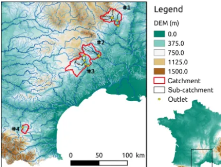
frame-Figure 1. Locations of the catchments studied, with a topo-graphic visualisation at a resolution of 25 m (Source – IGN; MNT BDALTI).

work, such as FUSE (Framework for Understanding Struc-tural Errors, Clark et al., 2008) or SUPERFLEX (Flexible framework for hydrological modeling, Fenicia et al., 2011). However, Clark et al. (2015a, b) have also proposed a uni-fied structure to test multiple working hypotheses within a distributed modeling framework. To our knowledge, the case studies using the aforementioned frameworks are related to continuous hydrological studies in order to assess hydrolog-ical hypotheses through the overall hydrologhydrolog-ical signature of the catchments. In this work, we extend the method of multi-ple working hypotheses to the assessment of an event-based hydrological model framework.

The objective is to test a number of proposed hydrologi-cal mechanisms that occur during flash flood events in a set of contrasting catchments in the French Mediterranean area. While the proportion of flows passing through the soil ap-pears to be significant, questions arise about how they form: – Are they subsurface flows that take place in a restricted

area of the root layer as a result of preferential path ac-tivation? Or are they lateral flows taking place at greater depth, comparable to those seen in some aquifers? – Does the geological bedrock or an altered substratum

play a role limited to that of mere storage reservoir, or is it actively involved in flood flows formation? – Which are the flow processes proportions, according to

the events and the catchments?

The aim of this article is to attempt to answer these ques-tions using a multi-model approach that tests different types of hydrological dynamics. The study was based on MA-RINE (Modélisation de l’Anticipation du Ruissellement et des Inondations pour des évéNements Extrêmes), a phys-ically based, distributed hydrological model (Roux et al.,

2011; Garambois et al., 2015a), which was developed specif-ically to model flash floods in the catchments of the French Mediterranean Arc. Several new representations for the soil column and underground flows were proposed (Douinot, 2016) and included in the MARINE model in the form of modules that can be used to test different hydrological func-tions (Sect. 3). Those different hydrological dynamics were applied to a set of catchments, presented in Sect. 2, with physiographic properties representative of the whole of the French Mediterranean Arc. The performance of each model was then examined and subjected to a comparative study (Sects. 4 and 5). The contributions of the results for improv-ing the hydrological functionimprov-ing understandimprov-ing are lastly dis-cussed in Sect. 6 before concluding.

2 Catchments and data used in the study 2.1 Study catchment set

We studied the behaviour of four catchments and eight nested catchments in the French Mediterranean Arc (Fig. 1). The catchments (in the order they are numbered in Fig. 1) were those of the Ardèche, Gard, Hérault and Salz rivers. These were selected for the following reasons; (i) they are represen-tative of the physiographic variability found in areas where flash floods occur, (ii) numerous studies of flash floods have already been carried out on the Gard and Ardèche (Ruin et al., 2008; Anquetin et al., 2010; Delrieu et al., 2005; Maréchal et al., 2009; Braud et al., 2014) that could guide the interpretation of the modelling results (Fenicia et al., 2014), and (iii) a considerable number of observations of flash flood events are available for these catchments.

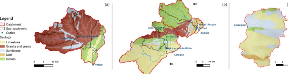
The main physiographical and hydrological properties of the catchments are presented in Table 1. Figure 2 shows the contrasting geological properties of the studied area; the catchments are marked by a clear upstream–downstream dif-ference. The Ardèche catchment upstream of Ucel essentially sits on a granite bedrock with some sandstone on its edges, while downstream the geology changes to predominantly schist and limestone formations. Similarly, the upstream part of the Gard catchment consists of schistose bedrock, while downstream the bedrock is impermeable marl-type and gran-ite formations. The Hérault catchment is split into mostly schist and granitic head watersheds (the Valleraugue and la Terrisse sub-catchments) and is a predominantly lime-stone plateau (Saint-Laurent-le-Minier sub-catchment). Fi-nally, the Salz is characterised by sedimentary bedrock com-prised of sandstone and limestone (Fig. 2).

Figure 2.The geology of the Ardèche catchment(a), the Gard and Hérault catchments(b), and the Salz catchment(c)(sources: BD Million-Géol, BRGM).

elling studies focused on this area (Garambois et al., 2013; Vannier et al., 2013) tend to support a hydrological classifica-tion according to those contrasting geological properties, in agreement with the usual hydrogeological signature found in the literature (Sayama et al., 2011; Pfister et al., 2017a). Marl, sandstone and limestone without karst are characterised by limited storage capacities, resulting in higher runoff coef-ficients and high sensitivity to the initial soil moisture (Ri-bolzi et al., 1997; Braud et al., 2016a). In contrast, in granite and schist transects located on the hillslope of the Ardèche catchment, infiltration tests and analyses of electrical resis-tivity signals show the high permeability of the geological substratum in depth (measured up to 2.5 m in depth); high storage capacities reach up to 600 mm in 7 out of 10 as-sessments with artificial forcing and the three remaining tests suggest local unaltered bedrock (Braud et al., 2016a, b). The natural resistivity profile suggests a regular soil bedrock in-terface when the latter consists of schist, while the granite one presents a more chaotic structure. Finally, the continuous comparative study of two experimental sites over surface ar-eas of the order of 1 km2– one located on the schist upstream part of the Gard catchment and the other one on the down-stream granite part – suggests that there is rapid subsurface flow processing on the schist area, while flow formation ap-pears to be controlled by the extension of the saturated zone related to the river on the granitic site (Ayral et al., 2005; Maréchal et al., 2009, 2013).

2.2 Forcing inputs and hydrometric data

The hydrometric data were derived from the network of oper-ational measurements (HydroFrance databank, http://www. hydro.eaufrance.fr/, last access: 10 May 2018). Eight to twenty years of hourly discharge observations were avail-able, according to the dates when the hydrometric stations were installed (Table 1).

Flood events with peak discharges that had exceeded the 2 year return period for daily discharge (QD2 in Table 1,

which corresponds to the alert threshold for flood

forecast-ing centres in France) were selected as events to be included in the study. Thus, only one criterion for hydrological re-sponse was considered. This led to a selection of precipita-tion events of varying origins (for instance, rainfall induced by mountains, stagnant convective cells and rainfall occur-ring in different seasons, mainly in autumn and early spoccur-ring). Such a selection risked complicating the study because flow processes can vary from one season to another. Nevertheless, it allowed us to test the ability of the model to deal with dif-ferent (non-linear) flow physics regimes. Note also that mod-erate or intense rainfall events without respective hydrologi-cal responses might be taken out of the analysis. Nevertheless the first alert threshold used here is small enough to have a selection of flood events with contrasting runoff coefficients (see Table 2).

E

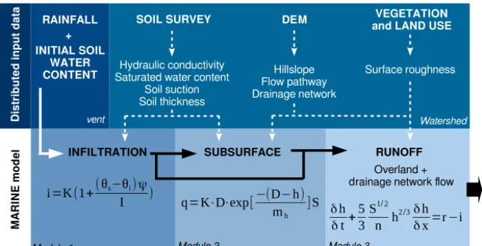
Figure 3.The MARINE model structure, parameters and variables. The Green–Ampt infiltration equation contains the following parameters: infiltration ratei(m s−1), cumulative infiltrationI(mm), saturated hydraulic conductivityK(m s−1), soil suction at the wetting front9(m), and saturated and initial water contents,θsandθi(m3m−3), respectively. Subsurface flow contains the following parameters: soil thickness

(m), lateral saturated hydraulic conductivityK(m s−1), local water depthh(m), transmissivity decay with depthmh(m) and bed slopeS (m m−1). The kinematic wave contains the following parameters: surface water depthh(m), timet(s), space variablex(m), rainfall rater (m s−1), infiltration ratei(m s−1), bed slopeS(m m−1) and Manning roughness coefficientn(m−1/3s). Module 2 described in this figure corresponds to the standard definition applied in the MARINE model.

As the MARINE model is event-based, it must be ini-tialised to take into account the previous moisture state of the catchment, which is linked to the history of the hydro-logical cycle. This was done using spatial model outputs from Météo-France’s SIM (Safran-Isba-Modcou, Habets et al., 2008) operational chain, including a meteorological anal-ysis system (SAFRAN; Vidal et al., 2010), a soil–vegetation– atmosphere model (ISBA; Mahfouf et al., 1995) and a hydro-geological model (MODCOU; Ledoux et al., 1989). Based on the work of Marchandise and Viel (2009), the spatial daily root-zone humidity outputs (resolution of 8 km×8 km) sim-ulated by the SIM conceptual model were used for the sys-tematic initialisation of MARINE.

3 The multi-hypothesis hydrological modelling framework

3.1 The MARINE model

The MARINE model is a distributed mechanistic hydrologi-cal model especially developed for flash flood simulations. It models the main physical processes in flash floods: infiltra-tion, overland flow and lateral flows in soil and channel rout-ing. Conversely, it does not incorporate low-rate flow pro-cesses such as evapotranspiration or base flow.

MARINE is structured into three main modules that are run for each catchment grid cell (see Fig. 3). The first mod-ule allows for the separation of surface runoff and infiltra-tion using the Green–Ampt model. The second module rep-resents the subsurface downhill flow. It was initially based

on the generalised Darcy’s law used in the TOPMODEL (TOPography-based) hydrological model (Beven and Kirby, 1979), but it was developed in greater detail as part of this study (see Sect. 3.2). Lastly, the third module represents overland and channel flows. Rainfall excess is transferred to the catchment outlet using the Saint-Venant equations sim-plified with kinematic wave assumptions. The model distin-guishes grid cells with a drainage network, where channel flow is calculated on a triangular channel section (Maubour-guet et al., 2007) from grid cells on hillslopes and where the overland flow is calculated for the entire surface area of the cell.

The MARINE model works with distributed input data such as (i) a digital elevation model (DEM) of the catchment to shape the flow pathway and distinguish hillslope cells from drainage network cells according to a drained area threshold, (ii) soil survey data to initialise the hydraulic and storage properties of the soil, which are used as parameters in the infiltration and lateral flow models, and (iii) vegetation and land-use data to configure the surface roughness parameters used in the overland flow model.

The MARINE model requires parameters to be calibrated in order to be able to reproduce hydrological behaviours ac-curately. Based on sensitivity analyses of the model (Garam-bois et al., 2013), five parameters are calibrated: soil depth, represented asCz, the saturation hydraulic conductivity used in lateral flow modelling,Ckss, the hydraulic conductivity at

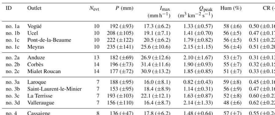
Table 2.Properties of the flash flood events as an average on the event set (±standard deviation). ID is the coding name of the concerned catchments (See Fig. 1: no. 1 for the Ardèche, no. 2 for the Gard, no. 3 for the Hérault and no. 4 for the Salz);Nevtis the number of observed

flash flood events;P (mm) is the mean precipitation;Imax(mm h−1) is the maximal intensity rainfall per event;Qpeakis the specific flood

peak (m3km−2s−1); Hum is the initial soil moil moisture according to SIM output (Habets et al., 2008); CR is the runoff coefficient (%).

ID Outlet Nevt P (mm) Imax Qpeak Hum (%) CR (–)

(mm h−1) (m3km−2s−1)

no. 1a Vogüé 10 192 (±93) 17.3 (±6.2) 1.33 (±0.57) 58 (±6) 0.50 (±0.16)

no. 1b Ucel 10 208 (±105) 19.1 (±7.1) 1.41 (±0.70) 56 (±5) 0.47 (±0.17)

no. 1c Pont-de-la-Beaume 10 222 (±122) 20.5 (±6.2) 1.79 (±0.82) 56 (±5) 0.51 (±0.22)

no. 1c Meyras 10 235 (±141) 25.6 (±10.6) 2.15 (±1.15) 56 (±4) 0.51 (±0.20)

no. 2a Anduze 13 182 (±69) 26.9 (±12.6) 2.10 (±1.67) 53 (±7) 0.31 (±0.13)

no. 2b Corbès 14 196 (±73) 31.4 (±11.6) 1.90 (±0.93) 55 (±7) 0.32 (±0.15)

no. 2c Mialet Roucan 14 177 (±72) 30.9 (±13.2) 1.85 (±0.85) 51 (±7) 0.33 (±0.15)

no. 3a Laroque 7 188 (±95) 16.0 (±8.1) 0.82 (±0.43) 59 (±8) 0.45 (±0.16)

no. 3b Saint-Laurent-le-Minier 7 153 (±95) 18.4 (±8.9) 1.14 (±0.31) 56 (±9) 0.47 (±0.16)

no. 3c La Terrisse 7 193 (±103) 22.1 (±12.1) 1.63 (±0.87) 52 (±8) 0.60 (±0.23)

no. 3d Valleraugue 7 156 (±110) 16.4 (±8.7) 2.14 (±1.33) 48 (±6) 0.62 (±0.22)

no. 4 Cassaigne 8 136 (±47) 17.8 (±6.2) 1.48 (±0.64) 57 (±7) 0.55 (±0.24)

drainage network.Ckss,Ck andCz are the multiplier coeffi-cients for spatialised, saturated hydraulic conductivities and soil depths. In this study, modifications of Module 2 (i.e. sub-surface downhill flow) were tested for assessing several pos-sible ways to represent the intra-soil hydrological function-ing. Consequently, instead of Cz andCkss, new parameters

of calibration were introduced, as described in the following section.

3.2 Modelling lateral flows in the soil: the development of a multi-hypothesis framework

We proposed several modifications to Module 2 – the subsur-face downhill flow submodel – covering the three hypotheses of hydrological functioning:

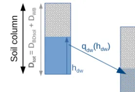
– The deep water flow model (DWF) assumed deep infil-tration and the formation of an aquifer flow in highly altered rocks. In hydrological terms the pedology– geology boundary was transparent. The soil column could be modelled as a single entity of depthDtot(m),

which is at least equal to the soil depth DBDsol(m)

(see Fig. 4). Given the lack of knowledge and avail-able observations, a uniform calibration was applied to the depth of altered rocks, represented asDWB(m),

which is rapidly accessible to the scale of a rain event. Groundwater flow was described using the generalised Darcy’s law (qdw, Eq. 1). The exponential growth of the

hydraulic conductivity at saturation as the water table (hdw) rises assumed an altered rock structure where

hy-draulic conductivity at saturation decreases with depth

(the TOPMODEL approach).

qdw=Kdw·Dtotexp

_h

dw−Dtot

mh

·S, (1)

withhdw(m)as the water depth of the unique water

ta-ble,mh(m)as the decay factor of the hydraulic

conduc-tivity at saturation with soil depth,S[-] as the bed slope,

Kdw=Ckdw·KBDsol(m s−1)as the simulated hydraulic

conductivity at saturation andDtot=DBDsol+DWBas

the soil column depth. Calibrated parameters are in bold.

– The subsurface flow model (SSF) assumed that the for-mation of subsurface lateral flows was due to the activa-tion of preferential paths, like the in situ observaactiva-tions of Katsura et al. (2014) and Katsuyama et al. (2005). The altered soil–rock interface acts as a hydrological bar-rier. The rapid saturation of shallow soils results in the development of rapid flows due to the steep slopes of the catchments and the existence of rapid water flows circulating through the macropores as the soil becomes saturated. The soil column was thus represented by a two-layer model (see Fig. 5), with the depth of an up-per layer equal to the soil depthDBDsol(m) and a lower

layer of uniform depthDWB(m). The lateral flows in the

upper layer were described by the generalised Darcy’s law. However, variations in hydraulic conductivity were expressed as a function of the mean water content of the layer (θsoil) and not of the height of water (hsoil) that

pref-erential paths in the soil by the increase in the degree to which the soil is filled. The decay factor of the hy-draulic conductivity as a function of the saturation rate,

mθ, was set according to the linearised empirical rela-tions developed by Van Genuchten (1980) between the hydraulic conductivity and soil water content for the dif-ferent classes of soil textures. Flows in the lower soil layer (qdw; Eq. 3) in the form of a deep aquifer were

limited by setting the hydraulic conductivity of the sub-stratum as being equivalent to that of the soil divided by 50 (this choice being guided by the orders of magni-tude generally observed in the literature; Le Bourgeois et al., 2016; Katsura et al., 2014). The altered rocks were thus assumed to mainly play a storage role. In-filtration occurring between the two layers was initially restricted by the Richards equations, which were incor-porated using the set hydraulic properties of the sub-stratum (Eq. 4). When the upper layer is saturated, this allows the filling through a piston effect. The depth of the soil layer,DBDsol, was set according to the soil data,

while the depth of the substratum,DWB, was calibrated

in the same way as in the DWF model.

qss=Kss·DBDsolexp

_θ

soil−1

mθ

·S, (2)

qdw=Kdw·DWBexp

_h

WB−DWB

mh

·S, (3)

qinf= −Kdw

δH (θsoil, θWB)

δz , (4)

wherehsoil andhWB(m) represent the soil water depth

in the upper and lower layer, respectively, θsoil and θWB (−) represent the soil water content of the upper

and lower layer, respectively,mθ (−) represents the de-cay factor of the hydraulic conductivity with soil water contentθsoil,Kss=Ckss·KBDsolandKdw=0.02·Kss

(m s−1) represents the simulated hydraulic conductivity at saturation of the upper and lower layer in the SSF model, respectively.

– The subsurface and deep water flow model (SSF-DWF) assumed that the presence of subsurface flow was due not only to local saturation of the top of the soil col-umn, but also to the development of a flow at depth, as a result of significant volumes of water introduced by infiltration and a very altered substratum whose appar-ent hydraulic conductivity was already relatively high. This hypothesis of the process led to a modelling ap-proach analogous to the SSF model (Fig. 5), where the hydraulic conductivity at substrate saturation,Kdw, was

no longer simply imposed, but instead was calibrated using an additional coefficient,Ckdw. In the SSF-DWF

model,

Kdw=Ckdw·KBDsol. (5)

Figure 4.DWF model of flow generation by infiltration at depth and support of a deep aquiferqdw(hdw)(Eq. 1).

Figure 5.SSF and SSF-DWF models of flow generation by the satu-ration of the upper part of soil column and activation of preferential paths (qss), with support flow at depth (qdw) and water exchanges

from the upper layer to the lower one according to both soil water content, represented byqinf(θsoil, θWB). See Eqs. (2), (3) and (4)

for the definition of the flows.

The soil water content prior to simulation was similarly initialised for each model in order to ensure that, for a fixed depth of altered rock, the same volume of water was allocated for all models. The SIM humidity indices (Sect. 2.2) were used to set an overall water content for all groundwater flow models for a given flood.

4 Methodology for calibrating and evaluating the models

4.1 Calibration method

The three hydrological models studied, DWF, SSF and SSF-DWF, were calibrated for each catchment by weighting 5000 randomly drawn samples from the parameter space for each model (the Monte Carlo method). The weighting was done using the DEC (Discharge Envelope Catching) score (Eq. 6; discussed by Douinot et al., 2017) in order to integrate the a priori uncertainties of modelling σmod, i, i=1. . .n

, as represented by Eq. (7), and those related to the flow mea-surements σyˆi

, i=1. . .n, as represented by Eq. (8). The

of floods in order to be able to forecast flash floods) while always being aware of the uncertainties in the reference flow measurements.

Given the lack of information, these uncertainties

σyˆi

, i=1. . .n were set at 20 % of the measured

dis-charge, which is in line with the literature on discharge mea-surements from operational stations (Le Coz et al., 2014), and increased linearly with the 10-year hourly discharge, beyond which, as a general rule, the observed flow is no longer measured but is derived by extrapolation from a dis-charge curve, making it less accurate (Eq. 8). The envelope

ˆ

yi±2σyˆi

, i=1. . .nconsequently defines the 95 %

con-fidence interval of the observed flows.

The modelling uncertainties σmod, i, i=1. . .n

were set at a minimum value (as a function of the basic catchment module), thus ensuring that the evaluation of the hydrographs would not be unduly affected by the reproduction of rela-tively low flows, which were strongly dependent on initiali-sation using previous moisture data that were not the subject of this study. In addition, it was assumed that a modelling un-certainty of 10 % around the confidence interval of observed flows was acceptable (Eq. 7). Finally, the overall overarching envelope yˆi±2σyˆi±2σmod, i

, i=1. . .ndefines hereafter

the acceptability zone, that is to say the interval in which any simulated flow would be considered as acceptable, according to the modelling and measurement uncertainty definitions.

DEC=1

n

n X

i=1

_iDEC=1

n

n X

i=1

di

σmod, i

, (6)

σmod, i=0.5·Q+0.025· ˆyi, (7)

σyˆi=0.05· ˆyi·

1+ yˆi

QH10

, (8)

with_iDECas the DEC modelling error at timei,yˆiandσyˆias the observed discharge and the uncertainty of measurement at timei,di as the discharge distance between the model pre-diction at timei(yi) and the confidence interval of observed flow at timei (yˆi±2σyˆi),σmod, ias the simulated uncertainty at timei, andQandQH10as the mean inter-annual discharge

and the 10 year maximum hourly discharge of the related catchment, respectively.

4.2 Metrics and key points in model evaluation and comparison

Results of the models were first assessed and benchmarked using performance scores (Sect. 5.1). The evaluation focused on the performance of the models in reproducing the hydro-graphs in overall terms but also more specifically on their ability to reproduce the characteristic stages of floods: ris-ing flood waters, high discharges and flood recession. These stages were defined as follows:

– The period of rising flood waters is between the moment when the observed flow rate exceeds the mean inter-annual discharge of the catchment and the date of the first flood peak.

– The stage of high discharges includes the points for which the observed flow was greater than 0.25 times the maximum flow during the event.

– The stage of flood recession begins after a period of

tc, which is the catchment concentration time

accord-ing to Bransby’s formula (Pilgrim and Cordery, 1992), represented bytc=21.3·L/(A0.1·S0.2)after the peak

of the flood, and ends when discharge is rising again (or, where appropriate, at the end of the event, which is the time of peak flooding+48 h).

The DEC score has provided a standard assessment of the modelling errors, enabling a reasonable weighting of the sim-ulations. However, for a sake of easy understanding, the per-centage of acceptable points of the simulated median time series, Qmed_INT [%] (Douinot et al., 2017), was chosen to evaluate the ability of the models to reproduce overall flows, rising flood waters and high discharges. A point is defined as acceptable when the median simulated value stands within the modelling acceptability zone yˆi±2σyˆi±2σmod, i

, i=

1. . .n

.

Conversely, Qmed_INT was not relevant for the evalua-tion of the capacity to reproduce recessions, because the cal-culation of this score during the recession interval strongly depends on performance at high discharges. Instead, we used theAslopescore defined in Eq. (9). It calculates the average

standard error in simulating the decreasing rate of the dis-charge during the flood recession interval. Through the con-sideration of theAslope score here, it was assumed that the

recession rate is a relevant feature of the catchment’s hydro-logic properties (Troch et al., 2013; Kirchner, 2009).

Aslope=

Pl

i=k|

dyi

dt −

dyˆi

dt| Pl

i=k

dyˆi

dt

, (9)

wheredyˆi

dt and

dyi

dt are the observed and the simulated reces-sion rates, respectively, at a time stepi that belongs to the flood recession interval i=k. . .l

.

The evaluation was completed through the descrip-tion of the modelling errors (Sect. 5.2) in order to identify those that were inherent in the choice of model structure, regardless of the calibration methodol-ogy adopted (Douinot et al., 2017). Attention was paid to the a priori and a posteriori confidence interval of the model simulations defined byy_iprior−5th, y_iprior−95th, i=

1. . .n and y_iDEC−5th, y_iDEC−95th, i=1. . .n,

percentile of the 5000 model simulation values at timei, and wherey_iDEC−5thandy_iDEC−95thare the 5th and the 95th per-centile of the same but weighted series according to the DEC calibration criterion.

Those confidence intervals were standardised according to the DEC modelling error definition (Eq. 6), defining the a priori and a posteriori confidence intervals of the modelling errors;

_iα−xth=

    

   

0 if |y_iα−xth|≤2·σyˆi

y_iα−xth±2·σyˆi

2·σmodi

otherwise

(−ify_iα−xth>0; +if y_iα−xth≤0)

(10)

whereα_i−xthis thexthpercentile of theαmodelling errors distribution at timei.

The latter definition allows for an informative transla-tion of the prior and posterior confidence intervals (Douinot et al., 2017); a value of_iα−xthequal to 0 indicates that the

y_iα−xthbound lies within the discharge confidence interval. If 0<_iα−xth≤1, they_iα−xthbound lies within the acceptability zone. If_iα−xthis larger than 1, the errors of modelling are de-tected or remain. In addition, the benchmark of both a priori and a posteriori confidence intervals allows for highlighting, which was the remaining modelling errors that were induced by the model’s assumptions and those that were induced by the calibration.

5 Results

5.1 Performance of the models

5.1.1 Overall performances of the models

Assessment of the performances by catchment. Fig. 6 shows the average and standard deviations of the Qmed_INT scores obtained after the calibration of the DWF, SSF and SSF-DWF models for each catchment studied. The SSF-DWF model, assuming deep infiltration and the formation of an aquifer flow in altered bedrock, showed better performance in the Ardèche catchment (no. 1), while in the Gard (no. 2) and the Salz (no. 4) catchments, the SSF and SSF-DWF models, assuming the formation of subsurface flows due to the ac-tivation of preferential flow paths by local saturation (SSF) with development of flow at depth (SSF-DWF), produced the most accurate results. On the Hérault catchment (no. 3), the modelling results obtained with each model in terms of Qmed_INT were less obvious, although the SSF-DWF model seemed to stand out to some extent. The differences in model performance were more pronounced for the valida-tion events. The better-performing models tended to be more consistent, with equivalent Qmed_INT scores on calibration and validation events, for example, the DWF model on the Ardèche (no. 1) or the SSF and SSF-DWF models on the

Events of calibration

no. 1a no. 1b no. 1c no. 1d no. 2a no. 2b no. 2c no. 3a no. 3b no. 3c no. 3d no. 4 Mean

Qmed_INT (%)

0

50

100

Assessment of all the hydrographs

DWF SSF SSF−DWF

Mean value Q5th − Q95th

Events of v

alidation

no. 1a no. 1b no. 1c no. 1d no. 2a no. 2b no. 2c no. 3a no. 3b no. 3c no. 3d no. 4 Mean

Qmed_INT (%)

0

50

100

(a)

(b)

Figure 6. Qmed_INT scores, with mean Qmed_INT scores ob-tained for the calibration(a)and validation(b)events, by model and catchment. The Qmed_INT scores were calculated for the whole hydrograph. Thexaxis refers to the ID number of each catchment (Fig. 1). Finally, the mean attribute refers to the average results over all the catchments obtained with each model.

Gard (no. 2). There was also a deterioration in performance in several models that had already been judged as less ef-fective, for example, the SSF and SSF-DWF models on the Ardèche (no. 1) or the DWF model on the two catchments of the Hérault, no. 3c and no. 3d.

SSF model versus SSF-DWF model. As a reminder, the dif-ference between the SSF and SSF-DWF models is that the latter has an extra calibration parameter,Ckdw, which is able

to initialise a significant lateral flow in the subsoil horizons of the soil column (see Eq. 3). The lateral hydraulic conduc-tivity in the deep layer is configured using the hydraulic con-ductivity from BDsol; Kdw=Ckdw·KBDsol, withCkdwset

to 0.02·Ckss in the SSF model and calibrated in the

SSF-DWF model. The small differences between the SSF and SSF-DWF models showed that this flexibility does not pro-duce any significant improvement, with the exceptions of the Ardèche catchment at Meyras and the Hérault catchment at Valleraugue. These two areas have a number of common fea-tures that could explain the similar modelling results; they are at the heads of high elevation catchments with steep slopes (Table 1) and are subject to considerable annual meteorolog-ical forcing. The calibration ofCkdwconsistently tended to

Module Q _0.01

0.05

no. 1a no. 1b no. 1c no. 1d no. 2a no. 2b no. 2c no. 3a no. 3b no. 3c no. 3d no. 4 Ckd

w

(−

)

0.01

0.05

(a)

(b)

.

Figure 7. (a): Mean inter-annual discharge (m3km−2s−1) for the catchments.(b): a posteriori distribution of the calibration of the subsoil horizon hydraulic conductivity in the SSF-DWF model (the Ckdwparameter; Eq. 3)

with exclusively higher values from the prior confidence in-terval having been selected (Fig. 7). In general, the calibra-tion of theCkdwparameter of the SSF-DWF model correlates

with the more or less sustained, annual hydrological activity of the catchments; the confidence interval of theCkdw

coef-ficient is restricted to low values for the catchments with low mean inter-annual discharges (no. 2a, no. 2b, no. 2c, no. 3a, no. 3b and no. 4) and inversely for the catchments with high mean inter-annual discharges (no. 1, no. 3c and no. 3d). 5.1.2 Detailed performances: assessment of the models

to simulate the different stages of an hydrograph Figure 8 shows the detailed assessments according to the specific stages of the hydrographs. It highlights whether the overall performances (Fig. 6) reflect uniform results along the hydrographs or if they actually hide the contrasting like-lihood of the simulations over the course of different hydro-graphs’ stages.

Uniform results are observed on the Gard catchment at Corbès and Anduze (no. 2a and no. 2b) and on the Salz catchment (no. 4); the SSF and SSF-DWF models demon-strated clearly superior performances for all stage-specific assessments of those catchments. For the Gard catchment at Mialet (no. 2c), the detailed assessment (Fig. 8) shows that the overall superiority of the SSF and SSF-DWF models is mainly due to a better simulation of the rising limb. Never-theless, for any score, the SSF and SSF-DWF models simi-larly both present the best modelling results compared to the DWF model.

On the Ardèche catchments (no. 1a, no. 1b, no. 1c and no. 1d), the overall performances reflect the simulation of the high discharges and of the flood recessions. There, the DWF model gives the best results for simulating those hydro-graphs’ stages. Conversely, it deals slightly less well with the simulation of the rising flood waters. As shown in Sect. 5.2,

all the models tend to underestimate initial flows prior to the event and during the onset of a flood. The DWF model, in particular, exhibits this modelling weakness; for example, see the onset of floods in the hydrographs for the 18 Octo-ber 2006 and 1 NovemOcto-ber 2014 events in Ucel (no. 1b) as depicted in Fig. 10, which explains the poorer performance. It can be noticed that the SSF-DWF model clearly better sim-ulated the rising flood waters of the Ardèche head watershed (no. 1d), explaining the overall good performance as well of this model on this catchment (Fig. 6).

On the Hérault, the detailed evaluation enabled us to dis-tinguish the performance of the different models. On the one hand, for the two larger catchments (no. 1a and no. 1b), the DWF model performed slightly better for rising flood wa-ters simulations, while the SSF model gave more clearly bet-ter simulations of the flood recessions. On the other hand, the SSF-DWF model generated the best simulations of the rising flood waters and of the high flows on the upstream catchments of La Terrisse (no. 3c) and Valleraugue (no. 3d), while the DWF model simulated a better flood recession. These contrasting results explained why there is not a spe-cific model that stands out on this catchment. In addition, it suggests a marked influence of the physiographic properties on the development of flow processes, because they are cor-related with the differences in the geological and topograph-ical properties of the Hérault (no. 3; see Fig. 2 and Table 1). The hydrological behaviours simulated for the Valleraugue and La Terrisse sub-catchments, which are predominantly granitic and schistose and where slopes are very steep, can be distinguished from those of Laroque and Saint-Laurent-le-Minier, which are mainly sedimentary and in the form of large plateaus.

5.1.3 Summary of the assessment

Figure 9 sums up the highlighted models according to the assessed hydrograph’s stage. It shows when one’s model has a clearly higher performance according to the following defi-nition; a model is assessed as clearly superior when the lower bound of the confidence interval of its score is higher than the median values of the scores obtained with the other models. It reveals that the catchments set might be divided into four groups:

– A first group of catchments is where the SSF and SSF-DWF models uniformly perform either similar or bet-ter than the DWF models. This is the case for the Gard (no. 2) and the Salz (no. 4) catchments.

Events of calibration

no. 1a no. 1b no. 1c no. 1d no. 2a no. 2b no. 2c no. 3a no. 3b no. 3c no. 3d no. 4 Mean

Qmed_INT (%)

0

50

100

(a) Assessment of the rising limbs

DWF SSF

SSF−DWF Mean value

Q5th − Q95th

Mean

Qmed_INT (%)

0

50

100

(b) Assessment of the high flows

Mean

Aslope

(−)

#1a #1b #1c #1d #2a #2b #2c #3a #3b #3c #3d #4

1.0

0.8

0.6

0.4

0.2

(c) Assessment of the recessions

Events of v

alidation

Mean

Qmed_INT (%)

0

50

100

Mean

Qmed_INT (%)

0

50

100

Mean

Aslope

(−)

1.0

0.8

0.6

0.4

0.2

no. 1a no. 1b no. 1c no. 1d no. 2a no. 2b no. 2c no. 3a no. 3b no. 3c no. 3d no. 4 no. 1a no. 1b no. 1c no. 1d no. 2a no. 2b no. 2c no. 3a no. 3b no. 3c no. 3d no. 4

no. 1a no. 1b no. 1c no. 1d no. 2a no. 2b no. 2c no. 3a no. 3b no. 3c no. 3d no. 4 no. 1a no. 1b no. 1c no. 1d no. 2a no. 2b no. 2c no. 3a no. 3b no. 3c no. 3d no. 4 no. 1a no. 1b no. 1c no. 1d no. 2a no. 2b no. 2c no. 3a no. 3b no. 3c no. 3d no. 4

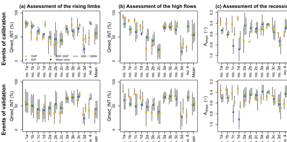
Figure 8.Assessment of the models by catchment in the different stages of the hydrographs.(a): Qmed_INT scores calculated over the rising flood waters stage.(b): Qmed_INT scores calculated over the high discharges stage.(c):Aslopescores. High Qmed_INT scores and

conversely lowAslopevalues indicate good performances of the model.

Figure 9. Summary of the models’ benchmark. A colour is at-tributed for each score and each catchment when one model gives a clearly superior performance, or two colours are attributed for each score and each catchment when two models give clearly superior performances: the score of a model is defined as clearly superior when the lower bound of its confidence interval is higher than the median values obtained with the other models. The superiority of a model might be half attributed if the criteria is only respected for the calibration processes. Colour attribution: orange for the DWF model, blue for the SSF model, green for the SSF-DWF model and grey when the superiority of one’s model is undetermined.

– A third group is where the models’ results are not really discernible. For those catchments, the DWF model ap-pears to simulate the rising flood and the high discharge slightly better, while the recession is better represented by the SSF model. This is the case for the downstream Hérault catchments (no. 3a and no. 3b).

– A last group is where the SSF-DWF model generates the rising flood and the high discharge slightly better, while the recession is better represented by the DWF

model. The head watersheds of the Hérault (no. 3c and no. 3d) and of the Ardèche (no. 1d) catchments are in this group.

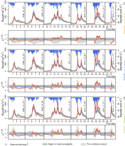
5.2 Modelling errors inherent in the models’ structures For the sake of conciseness, only the simulation over one catchment is presented. Figure 10 shows the simulation re-sults of the three models over the Ardèche catchment at Ucel (no. 1b). It shows the simulated hydrographs and their con-fidence intervals compared with the observed flows as well as the inherent errors in the simulations. This highlights the modelling errors due to the choice of model structure (DWF, SSF or SSF-DWF models). When the a priori confidence in-terval (grey colour) at a timeidoes not cross the acceptability region (green colour), it means that no parameter set gives an acceptable simulation, and modelling errors due to the structure (or assumptions) of the model are consequentially detected. When the posterior confidence interval (salmon colour) is outside the acceptability zone, the modelling error remains. Finally whether the prior (posterior) interval is large or small, the model’s structure allows for reaching a larger or less large range of simulated values (the model prediction is more or less uncertain, respectively).

the modelling errors is low at that point. More specifically, it tends to underestimate the initialisation discharges, because the variation interval of the errors over this period is predom-inantly negative. This may explain this model’s relative diffi-culty in reproducing the onset of floods, since the calibration of the parameters did not allow the acceptability zone in this part of the hydrograph to be reached. A resulting interpreta-tion applicable to the catchment sets is that good results in modelling the rising flood waters with the DWF model mean that the observed rising flow is relatively slow and could be reached in spite of the restrictive modelling structure (for ex-ample, no. 3aand no. 3b).

Likewise, it can be noted that the one-compartment struc-ture (i.e. the DWF model) allows for flexibility in the mod-elling of high discharges and flood recessions, because the confidence interval of the modelling errors is quite large over these periods in the hydrograph. However, it also led to the underestimation of high discharges and flood recessions. In fact, the prior modelling error interval (in grey) has a negative bias with respect to the acceptability zone. The calibration fi-nally allows the simulations to be selected at the intersection of the acceptability zones and the a priori confidence in mod-elling errors. This generally corresponds to the calibration of a low-depth altered rock,DWB, in order to make the model

more sensitive to soil saturation and more responsive via the generation of early runoff. From that resulting lowDWB, the

simulated water storage capacity is limited, which might ex-plain the inadequacy of the DWF model for a catchment with small runoff coefficients (no. 2, Table 2).

Conversely, the two-compartment structure (the SSF and SSF-DWF models) offers flexibility in modelling the begin-ning of events, flood warbegin-nings and high discharges, but the ability to model flood recessions is more constrained. SSF and SSF-DWF models simulate fast flood recessions in com-parison to the DWF model, suggesting that good results in modelling the flood recession with the SSF model that might be interpreted as a fast return to normal or low discharge are observed on the related catchments (as example, no. 2, no. 4). In the SSF and SSF-DWF models, the addition of a flux calibration parameter in the subsoil horizons not surprisingly leads to wider variations in the a priori modelling errors. A surprising finding, however, is that the calibration of the lat-eral conductivity of the deep layer,Ckdw, seems to affect only

the simulation at the beginning of the hydrographs (see the events of 1 November 2011 and 13 November 2014, Fig. 10) and has a very little effect on flood recessions. The high similarities of the prior modelling intervals of the SSF and SSF-DWF models explain the similar performances of those models. In the same way, when there is improvement in the performance through the SSF-DWF, it concerns the early ris-ing of the flood; as the detailed performances have already shown, the SSF-DWF enables the fast and early start of the flood events.

5.3 Analysis of relevance of the internal hydrological processes simulated

5.3.1 Characterisation of the hydrological processes simulated

The proportional volumes of the water making up the hydro-graphs, which arise from the three main simulated paths (on the surface, through the top or through the deep layer of the soil), were calculated. Figure 11 shows the simulated runoff contribution, i.e. the water that has not passed through the soil at any point. The contributions of these surface flows on the whole of the hydrograph (Fig. 11, left) and those that sup-port high discharges (Fig. 11, right) are distinguished. Note that the other contributions are not detailed, being correlated to the runoff assessment and therefore leading to a similar analysis.

The runoff contribution simulated by the DWF model even further discredits that model for representing the hydrologi-cal behaviour of the Gard (no. 2) and Salz (no. 4) catchments. Really high proportion of runoff contribution over the entire hydrograph were simulated, ranging from 40 % to 98 %. In contrast, the few experimental measurements made on the Gard (Bouvier et al., 2017; Braud et al., 2016a) provide evi-dence of the proportions of new water, which might be seen as an upper bound for runoff contribution volume, ranging from 20 % to 40 % of the volumes in the hydrograph. The SSF and SSF-DWF model conversely gave a more reason-able runoff contribution, although it remained high, ranging from 19 % to 62 %.

The assessment of the flow contributions through the most suitable model’s simulations for each catchment revealed in Sect. 5.1 is consistent with the catchment set’s diversity. Con-sidering the DWF model for the Ardèche catchment and the SSF and SSF-DWF models for the Gard catchment, the runoff contributions to the high flows of the hydrographs were slightly lower in the three downstream Ardèche catch-ments (no. 1a, no. 1b and no. 1c, with runoff contributions in-cluded between 17 % and 57 %) compared to the runoff con-tributions in the Gard catchment (no. 2a, no. 2b and no. 2c) and in the upstream part of the Ardèche (no. 1d, with runoff contributions between 20 % and 78 %). It is consistent with both the properties of the catchments and the rainfall forcing, with the first catchment subset (no. 1a, no. 1b and no. 1c) having deeper soil cover, a more permeable soil texture (see Table 1), and being forced by rainfall with lower maximal in-tensities (see Table 2), which is in contrast to the second one (no. 2a, no. 2b and no. 2c).

(a) Flow proportion of the whole hydrograph (b) Flow proportion in the high flows

no. 1a no. 1b no. 1c no. 1d no. 2a no. 2b no. 2c no. 3a no. 3b no. 3c no. 3d no. 4

DWF SSF SSF−DWF

0.0

0.4

0.8

Catchment

C surface (−)

no. 1a no. 1b no. 1c no. 1d no. 2a no. 2b no. 2c no. 3a no. 3b no. 3c no. 3d no. 4 Mean value Q5th − Q95th

0.0

0.4

0.8

Catchment

Figure 11.Proportion of surface runoff in the flows at the outlet. Left: The proportion over the whole hydrograph. Right: the proportion at high discharges (observed flow greater than 0.25 times the maximum flow during the event).

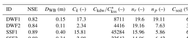
Table 3.Realistic models and parameter sets for the Hérault catchment at Saint-Laurent-le-Minier (no. 3b).Csoil: the contribution to the

hydrograph of flows passing through the soil.Ckdw/Ckss∗ : the value of the parameterCkdwfor model DWF (Eq. 1) or the value of the

parameterC_kss∗ for the model SSF (Eq. 2).

ID NSE DWB(m) Ck(–) Ckdw/C_kss∗ (–) nr(–) np(–) Csoil(%)

DWF1 0.82 0.15 17.3 8711 19.6 19.11 61

DWF2 0.84 0.11 2.34 4416 19.16 7.63 39

SSF1 0.89 0.40 15.81 45284 15.96 5.86 68

SSF2 0.89 0.34 2.08 22543 14.06 6.42 53

Notwithstanding the uncertainty related to the choice of the model when any model has been identified most suit-able through the performances, the largest uncertainties are related to the parameterisation of the models, a consequence of the equifinality of the solutions when calibrating a hydro-logical model against the sole criterion of the reproduction of the hydrological signal. While in terms of plausibility, sev-eral sets of parameters may be equivalent, even for the same model, these sets of parameters are likely to lead to a differ-ent hydrological functioning.

5.3.2 Detailed study of four plausible simulations on the Hérault watershed at Saint-Laurent-le-Minier

Spatialised and integrated changes in moisture levels and flow velocities generated within the catchments have been considered in order to give new details on the different im-pacts of the models’ structure, but also to explain the re-sulting uncertainty when assessing the flow processes’ dis-tribution. Next, the results of four simulations are described and are equally considered to be plausible according to the DEC criterion obtained from the DWF and SSF models (two simulations per model, see Table 3). The Hérault catchment at Saint-Laurent-le-Minier (no. 3b) has been considered be-cause of the equivalence of the models in representing that

catchment. Figure 12 compares the changes over time in the state of soil saturation and the different simulated flow veloc-ities of the four model+parameter setconfigurations (Ta-ble 3). Figure 13 compares the spatial distributions of these variables at a given moment.

In terms of hydrographs, which is quite logical given the similar likelihood scores, the simulations differed very little. The notable difference in the generation of hydrographs is the contribution of the different simulated flow paths. The pro-portions of water passing through the soil column (via sub-or surface-soil hsub-orizons) were highly variable, with an aver-age of 39 % for the DWF2 model, 53 % for the SSF2 model, 61 % for the DWF1 model and 68 % for the SSF1 model (Ta-ble 3). This is both due to (i) the structural choices (DWF and SSF) that involved a different saturation dynamics and the in-corporation of different types of flow, and to (ii) the choice of the parameters that involved flow velocities of different orders of magnitude.

(a) Hydrograph at Saint-Laurent-le-Minier

20/10/09 22/10/09 02/11/11 03/11/11 05/11/11 06/11/11 05/03/13 07/03/13 12/03/11 14/03/11 15/03/11 17/03/11 18/03/11

19:00 07:00 01:00 13:00 01:00 13:00 16:00 04:00 12:00 00:00 12:00 00:00 12:00

0

200

600

R

un

of

f (m

s

)

3

40

20

0

R

ai

nf

al

l (m

m

h

)

|

Obs. Y^

Sim. Y Subsurface Rainfall

(b) Mean soil moisture dynamic of the catchment

50

70

90

Humidity (%)

20/10/09 22/10/09 02/11/11 03/11/11 05/11/11 06/11/11 05/03/13 07/03/13 12/03/11 14/03/11 15/03/11 17/03/11 18/03/11

19:00 07:00 01:00 13:00 01:00 13:00 16:00 04:00 12:00 00:00 12:00 00:00 12:00

Upper soil compartment Soil column

(c) Mean subsurface velocities in the catchment

20/10/09 22/10/09 02/11/11 03/11/11 05/11/11 06/11/11 05/03/13 07/03/13 12/03/11 14/03/11 15/03/11 17/03/11 18/03/11

19:00 07:00 01:00 13:00 01:00 13:00 16:00 04:00 12:00 00:00 12:00 00:00 12:00

0.0

0.2

0.4

V

el

oc

iti

es

(c

m

s

)

-1

DWF1

DWF2 SSF1SSF2

(d) Mean runoff velocities in the catchment

20/10/09 22/10/09 02/11/11 03/11/11 05/11/11 06/11/11 05/03/13 07/03/13 12/03/11 14/03/11 15/03/11 17/03/11 18/03/11

19:00 07:00 01:00 13:00 01:00 13:00 16:00 04:00 12:00 00:00 12:00 00:00 12:00

0

5

10

20

V

el

oc

iti

es

(c

m

s

)

2009_10_18 * _{2011_11_01 **} 2013_03_05 * 2011_03_12 *

(e) Mean runoff velocities in the drainage network

20/10/09 22/10/09 02/11/11 03/11/11 05/11/11 06/11/11 05/03/13 07/03/13 12/03/11 14/03/11 15/03/11 17/03/11 18/03/11

19:00 07:00 01:00 13:00 01:00 13:00 16:00 04:00 12:00 00:00 12:00 00:00 12:00

0

40

80

120

V

el

oc

iti

es

(c

m

s

)

-1

-1

-1

-1

model produced a greater contrast in saturation levels be-tween different areas of the catchment (Fig. 13a and d). With the SSF model, the overall catchment saturation level was more related to the topography; saturated cells were observed close to the drainage network, and, lower water content was conversely observed in the upper reaches of the catchments. In fact, for the SSF model, rainfall forcing is mainly involved in the saturation of the upper soil layer (the dashed lines in Fig. 12b), which reacts very rapidly to precipitation.

As a result of the contrasting soil moisture dynamic, the flow velocities simulated in the soil showed consecutive dif-ferences. At the start of flooding, the SSF structure resulted in an early increase in flow velocities due to a higher and more homogeneous saturation level of the upper soil layer (Fig. 12c). Conversely, in the DWF model that simulated a more heterogeneous spatial saturation of the catchment, the simulated velocities increase was delayed, and the maximum values reached were 2 to 4 times lower.

The dynamics in the drainage network were impacted by the choice of the structure as well. The runoff velocities’ av-erage reflected the earlier inlet of the subsurface flow pro-cesses through the fast saturation of the upper compartment with the SSF model (Fig. 12e). The DWF model yields a more contrasting variation in the runoff velocities in the drainage network, mirroring variations in soil saturation lev-els.

The choice of parameters mainly implied different ranges of values for the velocities simulated in the soil, on the sur-face of the hillslope and in the drainage network. The cal-ibration of the CkssandCkdwparameters controlled the

or-der of magnitude in the subsurface velocities (Table 3 and Fig. 13b, e, h and k). The calibratedCk(infiltration capacity control) andDWB(depth of the subsoil horizon) parameters

controlled the infiltration as well, leading to a higher or less high number of cells with excess saturation or the infiltration capacity being reached (Fig. 13c, f, i, l) and consequently to a higher or less high proportion of runoff over the hillslope (Fig. 12d).

Several orders of magnitude were actually allowed while respecting the calibration objective, because the transit times of the different water pathways compensate each other. As foreshadowed by those four configurations, the selection of plausible parameter sets for any model in any catchment shows (i) a positive correlation between the parameters Ck and nr and np, suggesting the necessity of slowing down flows in the drainage network when a larger proportion of runoff from the catchments is simulated (i.e low Ck would imply lownr andnpand vice versa) and (ii) a positive cor-relation between Ck,CkssandCkdwparameters, suggesting

the necessity of accelerating the intra-soil flows when high infiltration rate is allowed and, consequentially, when larger proportion of subsurface flow is simulated. Thus, a degree of compensation occurs in the simulated transfer times between the various water paths from the hillslopes to the drainage network and from the drainage network towards the outlet.

6 Discussion

6.1 On the hydrological functioning of the catchments studied

The benchmark of the models’ performance on the catch-ment set leads to reveal four subsets, suggesting four dis-tinct hydrological behaviours. According to the modelling assumptions (Sect. 5.1), the resulting errors in simulating the different stages of the hydrographs (Sect. 5.2) and the catch-ment properties (Sect. 2.1), the hydrological behaviour of the catchment can be interpreted by each subset as follows:

– The SSF and SSF-DWF models showed better overall performance (with no particular pattern) in the first sub-set, the Gard (no. 2) and Salz (no. 4) catchments. This suggests, on the one hand, rapid catchment reactivity with fast rising flood waters as well as a fast flood reces-sion, and on the other hand, the formation of the flows in the soil through local saturation tied to the climate forcing. Although the models exhibited similar perfor-mances, the contrasting physiographic characteristics of these catchments suggest that there are different expla-nations for this better fit of the SSF-DWF model. On the Gard, the very high intensities of the observed events (Table 2) and/or the low soil depth (Table 1) may ex-plain the limitations on vertical infiltration due to the properties of the soil and/or geological bedrock. As a result, the rapid formation of a saturated zone at the top of the soil column favours runoff and a subsurface flux by activating preferential paths in the soil. This interpre-tation is in agreement with the field studies achieved on a schist upstream sub-catchment of the Gard, the schist substratum being the predominant geology of the Gard catchment (see Sect. 2.1, Ayral et al., 2005; Maréchal et al., 2009, 2013). On the one hand, on the Salz (no. 4), the soil is deeper and the precipitation intensities lower. On the other hand, the geological bedrock composed of marl, sandstone and limestone is assumed to have low permeability, and the soil is less conductive due to its predominantly silt-loam texture. As a result, despite the lower forcing intensities, the surface soil can reach sat-uration, which might explain why the SSF model offers the best fit.

a granite experimental sub-catchment localised in the downstream part of the Gard (Sect. 2.1, Ayral et al., 2005; Maréchal et al., 2009, 2013), the Ardèche catch-ment being granitic. The somewhat delayed flood ting that the structure of the one-compartment model im-posed seems to indicate that there are more rapid flows at the beginning of an event, which this model structure is not able to represent. A plausible explanation is the default calibration, which uses a uniform depth of ac-tive subsoil horizons,DWB, during a flood. This might

mask the appearance of local saturation zones and the subsequent runoff due to shallow soil and discontinu-ities in the permeable base layer (for example, in the downstream sedimentary layers, where infiltration tests have shown the appearance of runoff; see Sect. 2.1). In contrast, the SSF and SSF-DWF models did not display this weakness because the varying nature of soil depths (DBDsol, which determines the depth of the upper

com-partment) allowed for the rapid development of flows via preferential paths in the soil blocks, thus enabling the simulation of such local dynamics.

– The third subset consists of the downstream part of the Hérault (no. 3a and no. 3b). The models’ performances contrasted with the Hérault catchment heads (no. 3c and no. 3d), suggesting hydrological behaviours related to the contrasting geological properties. An interpretation of hydrological functioning is nevertheless not possible, given the similar overall results offered by the models and that no distinctions can be drawn according to other criteria.

– The last subset consists of the catchment heads (no. 1d, no. 3c, and no. 3d). We observed superior performances from the DWF and SSF-DWF models, with a particu-lar improvement in the forecasting of rising flood wa-ters when using the SSF-DWF model. This suggests the presence of several types of flow in the soil with strong support from flows at depth, which corroborates the high mean inter-annual discharges associated with these catchments, and additionally the presence of rapidly formed flows, providing a good simulation of the rising flood waters. The fact that the model SSF-DWF, which precisely alleged to represent the simultaneous setting up of shallow and deep subsurface flows, did not com-pletely outperform the two other models is interesting. From our point of view, it points out the limit of their artificial implementation, using a threshold infiltration from the top layer to the deep one. In reality, the simul-taneous setup of the two fluxes more likely refers to the spatial heterogeneity of the soil properties, especially in the head watersheds within a catchment cell (2.5 km2), which might allow either deep infiltration or fast topsoil saturation.

6.2 Overcoming the remaining uncertainty

The submitted multi-hypothesis test classically faced the equifinality issue related to the parameter uncertainty and highlighted the uncertainty related to the model’s structure. The comparative and detailed description of the simulation revealed the model’s structure controls, thus giving almost direct guidelines to overcome the equifinality issue.

One of the objectives of the study, the assessment of the flow contributions to the hydrographs, is not com-pletely reached, mainly because of the parameter uncertainty (Sect. 5.3.1). The benchmark of modeling configurations, scanning the different simulated processes (Sect. 5.3.2), showed how the calibration lead to that uncertainty. The wide range of values that has been allowed through the parame-ter setup enabled counparame-terbalancing effects between the inparame-ter- inter-nal velocities simulated. As a direct consequence, variable flow contributions could be simulated while finally produc-ing similarly likely hydrographs. This points out direct fur-ther objectives for improving and better restraining the cali-bration of the models. While several ranges of value for the internal flow velocities have been simulated, a reasonable restriction based on the velocity likelihood could be fore-seen. This further perspective should also shift experimental studies toward a better assessment of the water transit time along the different pathways at the hillslope scale, either us-ing direct methods such water isotope tracus-ing (Tetzlaff et al., 2018), developing imaginative indirect ones such as the di-atom tracing (Pfister et al., 2017b), or taking advantage of suspended particles and water turbidity measurements.