Drainage area characterization for evaluating green infrastructure using the Storm Water Management Model

(1)

https://doi.org/10.5194/hess-22-2615-2018 © Author(s) 2018. This work is distributed under the Creative Commons Attribution 3.0 License.

Drainage area characterization for evaluating green infrastructure

using the Storm Water Management Model

Joong Gwang Lee1, Christopher T. Nietch2, and Srinivas Panguluri3

1_{Center for Urban Green Infrastructure Engineering (CUGIE Inc), Cincinnati, OH 45255, USA}

2_{Office of Research and Development, US Environmental Protection Agency, Cincinnati, OH 45268, USA} 3_{Independent Consultant, Olney, MD 20832, USA}

Correspondence:Joong Gwang Lee ([email protected]) Received: 21 March 2017 – Discussion started: 19 May 2017

Revised: 22 March 2018 – Accepted: 3 April 2018 – Published: 3 May 2018

Abstract.Urban stormwater runoff quantity and quality are strongly dependent upon catchment properties. Models are used to simulate the runoff characteristics, but the output from a stormwater management model is dependent on how the catchment area is subdivided and represented as spa-tial elements. For green infrastructure modeling, we sug-gest a discretization method that distinguishes directly con-nected impervious area (DCIA) from the total impervious area (TIA). Pervious buffers, which receive runoff from up-gradient impervious areas should also be identified as a sep-arate subset of the entire pervious area (PA). This separa-tion provides an improved model representasepara-tion of the runoff process. With these criteria in mind, an approach to spa-tial discretization for projects using the US Environmen-tal Protection Agency’s Storm Water Management Model (SWMM) is demonstrated for the Shayler Crossing water-shed (SHC), a well-monitored, residential suburban area oc-cupying 100 ha, east of Cincinnati, Ohio. The model relies on a highly resolved spatial database of urban land cover, stormwater drainage features, and topography. To verify the spatial discretization approach, a hypothetical analysis was conducted. Six different representations of a common ur-banscape that discharges runoff to a single storm inlet were evaluated with eight 24 h synthetic storms. This analysis al-lowed us to select a discretization scheme that balances com-plexity in model setup with presumed accuracy of the out-put with respect to the most complex discretization option considered. The balanced approach delineates directly and indirectly connected impervious areas (ICIA), buffering per-vious area (BPA) receiving imperper-vious runoff, and the other pervious area within a SWMM subcatchment. It performed

well at the watershed scale with minimal calibration effort (Nash–Sutcliffe coefficient =0.852;R2=0.871). The ap-proach accommodates the distribution of runoff contributions from different spatial components and flow pathways that would impact green infrastructure performance. A developed SWMM model using the discretization approach is calibrated by adjusting parameters per land cover component, instead of per subcatchment and, therefore, can be applied to relatively large watersheds if the land cover components are relatively homogeneous and/or categorized appropriately in the GIS that supports the model parameterization. Finally, with a few model adjustments, we show how the simulated stream hy-drograph can be separated into the relative contributions from different land cover types and subsurface sources, adding in-sight to the potential effectiveness of planned green infras-tructure scenarios at the watershed scale.

1 Introduction

(2)

implement controls as close to the source of runoff genera-tion as possible (Debo and Reese, 2002; WEF-ASCE, 2012). Green infrastructure (GI) practices were developed to cor-rect this water pollution problem and restore the natural hy-drologic cycle (WEF-ASCE, 2012; USEPA, 2014). GI in-cludes structures like green roofs, rain barrels, bioretention areas, buffer strips, vegetated swales, permeable pavements, and infiltration trenches, or practices, such as disconnect-ing downspouts. The specific design objectives for GI in-clude minimizing the impervious areas directly connected to the storm sewer, increasing surface flow path lengths or time of concentration, and maximizing on-site depression storage and infiltration at the lot level (WEF-ASCE, 2012). This translates operationally to individual stormwater man-agement practices that are relatively small but densely dis-tributed in space (USEPA, 2009). Although GI is disdis-tributed at higher spatial densities, each unit is relatively inexpensive if the unit can be considered as part of landscaping and, in total, may provide a cost-effective alternative to more tradi-tional larger centralized practices, like detention ponds espe-cially in cases where land is not available or very expensive. There is a great deal of interest in modeling GI effects at watershed scales to help inform regional stormwater man-agement planning and design decisions. However, from a stormwater modeling perspective, the approach taken for model representations of GI requires different methodologi-cal considerations compared to the traditional large-size, low spatial density of the more centralized and regional control features (Fletcher et al., 2013; USEPA, 2012; Guo, 2008). While conventional stormwater management practices have focused on end-of-pipe controls at the downstream end of the drainage area (i.e., centralized systems), GI practices fo-cus on on-site controls at the upstream side (i.e., distributed systems). The surface hydrologic properties (e.g., land cover, slope, overland flow path) remain the same before or after ap-plying centralized systems, but they are altered with on-site GI systems. GI practices aim to amend the landscape hydro-logic properties to reduce the negative impacts of stormwater (USEPA, 2007). Hence, modeling approaches for evaluating GI should be able to account for the changing surface hydro-logic properties that come with GI implementation.

The Storm Water Management Model (SWMM) of the United States Environmental Protection Agency (USEPA) is one tool that has a large user base and a broad applica-tion history for informing stormwater management projects around the world (Niazi et al., 2017). In the current version of the model, GI effects are simulated using low-impact devel-opment (LID) algorithms. LID is largely synonymous with GI in SWMM vernacular. The LID modeling options were added in 2010 (Rossman, 2015; Rossman and Huber, 2016). Since then, while numerous LID/GI modeling studies have been introduced, best modeling practices for simulating GI in SWMM have received comparatively little attention in the literature (Niazi et al., 2017).

This study was intent on evaluating approaches to mod-eling GI effects at a watershed scale using SWMM. In the setup of a SWMM model, the urban area of interest is di-vided into smaller spatial units, referred to as subcatchments. To implement a traditional stormwater control feature like a retention pond, it is usually acceptable to provide mini-mal detail of the drainage area (Rossman and Huber, 2016). This leads to spatial aggregation which tends to produce larger subcatchment areas that aggregate land cover types and simplify the existing storm sewer system to realize a more cost-effective model setup and output data manage-ment. If the simulated hydrographs are matched with the ob-served data during model calibration, the model is considered a sound representation of the drainage processes important for designing the retention pond. The trade-off is that coarser schematization requires more decisions on how to aggregate catchment properties (Rossman and Huber, 2016). In con-trast, for simulation of GI, the construction reality is that GI is built as part of building and landscape arrangements all upgradient of the drainage network (Dietz, 2007; Montalto et al., 2007; USEPA, 2009; Zhou, 2014). Therefore, to accu-rately examine GI alternatives, a drainage area for modeling should be defined as an area that drains runoff to a storm sewer inlet with no or minimal spatial aggregation of land-scape features affecting hydrologic properties. In SWMM, this drainage area is modeled as single or multiple subcatch-ments. Since SWMM version 4.4H, overland flow routing is allowed from one subcatchment to another (Huber, 2001; Huber and Cannon, 2002). To minimize confusion between real and modeled drainage areas, we coin the term hydro-logic response element (HRE) in this study. An HRE is the drainage area (i.e., a real spatial element of the landscape being modeled) where GI practices may be implemented to control the element’s surface runoff prior to discharge to the stormwater collection system. There are many alternatives for configuring the HRE for GI modeling in SWMM. We evaluate six different options in this study.

(3)

proper-ties, surface runoff processes, and flow pathways within the HRE. Each subarea may also consist of different land cover components. For example, DCIA may include paved streets, building rooftops, driveways, or sidewalks. In this study, we questioned how these spatial and hydrologic realities should be modeled using SWMM.

After the HRE delineation is performed in SWMM, each HRE undergoes a model parameterization procedure that de-fines the relative proportions of impervious and pervious subareas, how they interact in terms of surface flow path-ways, and their hydrologic properties (Rossman, 2015). The subcatchment/subarea configuration of each HRE ultimately specifies the physical conditions used by the model’s math-ematical algorithms to simulate the dynamics of hydrologic loading to the drainage network. The more subcatchments there are, the more input and output values there are to be managed by the modeler. When setting up a SWMM model using the conventional objectives, such as deriving hydrographs for designing storm collection systems and/or detention–retention systems, the subcatchment parameteri-zation remains the same before and after simulation of the management practice; however, for GI simulation, the inter-nal properties of a subcatchment change, as mentioned ear-lier. Pending the type of GI, changes may need to be made to the hydrologic properties of subareas or individual land cover components, the proportions of impervious and pervi-ous area, the specification for the routing of runoff between them, the flow path length, and infiltration or the depres-sion storage properties. Adequately rationalizing and track-ing these changes can become a problem for the modeler when the total area being modeled is relatively large and ag-gregated, the GI scenarios are not the same among HREs, or the internal properties among HREs are heterogeneous. A systematic approach to characterizing HREs would help make SWMM GI simulation projects more efficient.

The question of how to best parameterize SWMM is not new, especially when it comes to spatial resolution and scaling, but as mentioned, GI modeling, in particular, re-quires special considerations. This paper describes a sug-gested method for modeling GI in SWMM and provides crit-ical evaluation. Primary objectives of this study are to (1) examine how to configure HREs for GI modeling and (2) develop a methodology for parameterizing a SWMM model that reflects this configuration with the goal of demonstrat-ing an urban watershed spatial discretization approach that optimizes model performance in terms of tracking model in-put values and presumed accuracy of the results. We hypoth-esized that conventional modeling approaches to subcatch-ment delineation are likely aggregating at too-coarse resolu-tion in space and hydrologic response to be appropriate for highly spatially distributed modern GI. We also questioned how the SWMM setup could not only allow for modeling the effects of various GI scenarios, but also facilitate the scal-ing of GI scenarios from a small HRE, representscal-ing the par-cel or lot level, to a watershed level. To answer these

ques-tions, we examine several acceptable approaches to repre-senting spatial reality in SWMM when the modeling objec-tive is to inform decisions about GI implementation. We use a hypothetical HRE-based analysis of spatial discretization alternatives to test our hypothesis related to the appropriate-ness of spatial and hydrologic response resolution. The hypo-thetical HRE represents a typical residential area that drains to a storm sewer inlet. The hypothetical HRE is modeled in SWMM by combining six conceivable options in spatial representation and eight design storms that represent the full spectrum of runoff events. From this analysis, an appropriate option is selected for GI modeling in SWMM, and a base-line SWMM model is developed using it for representing the existing condition of a well-characterized 100 ha urban wa-tershed in a headwater area east of Cincinnati, Ohio. To ex-amine the proposed approach, another SWMM model is de-veloped for simulating a GI implementation scenario at the study watershed. Also, an approach for hydrograph separa-tion is presented using the developed SWMM models, which can provide insight for arranging GI implementation scenar-ios. Currently, there is no provision for accomplishing this in SWMM.

2 Materials and methods 2.1 Study area

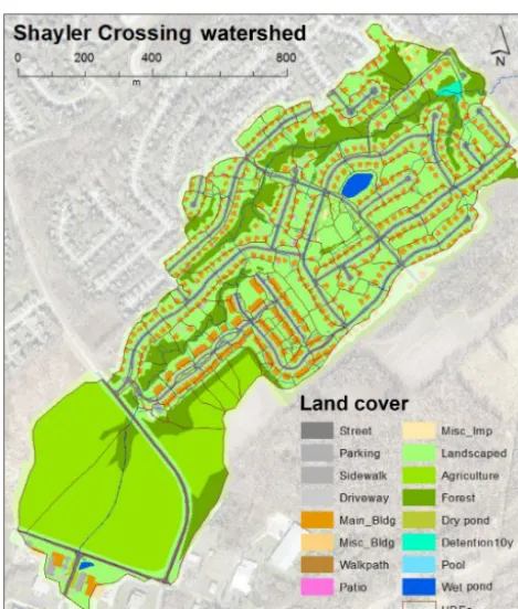
An experimental urban watershed drained by a natural head-water stream that does not have any surface stormhead-water in-flows from outside its topographic boundaries was used for this study (Fig. 1). The Shayler Crossing watershed (SHC) is located east of Cincinnati, Ohio, and occupies approximately 100 ha that is characterized as 62.6 % urban or developed, 25.6 % agriculture, and 11.8 % forested based on the 2011 National Land Cover Database (Homer et al., 2015). The na-tive soils of the watershed are characterized with high silty clay loam content and therefore are naturally poorly infiltrat-ing.

2.2 The baseline spatial database 2.2.1 Data from the county GIS

(4)

[image:4.612.52.280.66.209.2]

Figure 1.Location of the Shayler Crossing watershed. I-275 is an interstate highway around the Cincinnati metropolitan area.

the stormwater infrastructure like in this watershed are not always available to the modeler. In these cases, to adopt the subsequently described approach to GI scenario modeling in SWMM could require considerable ground-truthing and site surveying. In lieu of on-site visits, and as will become apparent from the descriptions below, what would be most important is determining the spatial location of storm sewer inlets. These are often visible from readily available aerial photographs; note that the visibility depends on the underly-ing image quality and the presence of obstacles such as trees or cars. When elevation data for the storm sewer network is unavailable, much can be inferred using surface elevation data and assuming local construction codes for stormwater infrastructures were applied, such as catch basin depths and conveyance pipe diameters and slopes. Such approximations would suffice for GI scenario analysis considerations and where storm sewer design is not the primary focus.

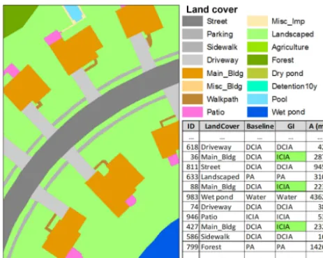
2.2.2 Detailed land cover and subarea categorization To obtain a high-resolution digital characterization of spa-tial reality in the study watershed, 16 unique land cover types were identified and digitized using ArcGIS 10.2 (ESRI, 2013) spatial analysis tools on the aerial orthophotographs of the study area. These 16 types are later aggregated to 10 for setting up the watershed SWMM model (see Ap-pendix). The resulting baseline spatial database included in-dividual records of the watershed surface that could be used to access the location, pattern, and extent of the following sixteen land cover types: streets, parking areas, sidewalks, driveways, main buildings, miscellaneous buildings, paved walking paths, patios, other miscellaneous impervious ar-eas, landscaped or lawn arar-eas, agriculture, forest, dry ponds, stormwater detention area (in SHC this is created by the addi-tion of a control structure to the stream channel itself), swim-ming pools, and wet ponds. Each spatial record has its own attributes (i.e., fields in the database) representing the cur-rent conditions (e.g., area, land cover) and was characterized

based on its future potential for GI implementation (e.g., to evaluate the potential of downspout disconnection for a main building). The initial parameterization and GI modeling ap-proaches described below for the SWMM model are based on content extracted from this land cover database created using ArcGIS tools. This database is often reused to perform model adjustments during calibration and GI scenario anal-ysis. The developed land cover database for SHC contains a total of 3682 records and the median area of each record is 23.5 m2.

Each surface record in the database is further classified into four types based on its hydrologic characteristics includ-ing (1) DCIA, (2) ICIA, (3) pervious area (PA), or (4) wa-ter. The PA is subsequently split into two subcategories called BPA and SPA after the HRE delineation procedure for SWMM modeling is completed (see below). All main buildings are DCIA because the rooftop downspouts in the existing condition are plumbed to directly discharge to the stormwater collection system through buried pipes or street gutters. All the miscellaneous buildings (e.g., storage sheds) are considered ICIA. Streets with curb-and-gutter drainage systems are identified as DCIA. Any directly connected up-gradient impervious areas to these streets are initially consid-ered as DCIA. These areas include directly connected drive-ways, parking areas, and sidewalks. However, if both sides of a sidewalk are surrounded by a pervious area, the side-walk is categorized as ICIA. Streets without curb-and-gutter drainage are ICIA. The remaining miscellaneous impervious areas are ICIA.

Figure 2 contains a sample GIS representation of the 16 land cover types along with a corresponding attribute table, which indicates hydrologic characteristics representing the baseline classification and a GI scenario-related classifica-tion. In the attribute table shown in Fig. 2, the first column contains the record identifier, the second column defines the land cover type, the third column defines how it was classi-fied for modeling the baseline condition, the fourth column defines how it was classified or reclassified for modeling a specific GI scenario, and the fifth column specifies the con-tributing area. For example, the record ID 36 contained in the table is initially classified as DCIA, but, after the rooftop drains were disconnected in the modeled GI scenario, the unit was reclassified as ICIA (in the fourth column). This methodology allows for GI-related hydrology evaluation to be performed without impacting the overall SWMM model structure and setup. A companion USEPA report (Lee et al., 2017) has been prepared to provide the relevant details on the applied spatial analysis techniques such as clip, intersect, union, buffer, and manipulating attribute data.

2.2.3 Configuring the BPA and SPA

(5)

re-Figure 2.Sample GIS classified representation of the land cover and hydrologic characteristics.

ceive a certain percentage of runoff from impervious areas; this is how ICIA is distinguished from DCIA. However, in reality, not all of the PA receives runoff from ICIA, rather just the part of the PA that is immediately adjacent to the ICIA. When evaluating GI scenarios, one strategy might be to enlarge the size of the buffering area adjacent to ICIA, or engineer GI structures (e.g., cascading filtering or biore-tention systems) around this buffering area (a.k.a. BPA) to reduce the direct runoff from impervious surfaces by routing them over grassy areas to slow down runoff and promote soil infiltration. Draining paved areas onto porous areas can re-duce runoff volumes, rates, pollutants, and cost for drainage infrastructure (NRC, 2009; WEF-ASCE, 2012). Therefore, because of the nuanced, yet important differences, in the geospatial relationship of PA in different GI scenarios, we rationalized the need for retaining the ability to model this aspect while evaluating GI scenarios by splitting the PA into BPA and SPA for GI modeling in SWMM.

[image:5.612.312.542.65.292.2]

Characterizing the precise “physical” extent of BPA is a complicated process that would have to be defined from highly resolved surface topography around ICIA and an un-derstanding of the unsaturated zone processes such as how infiltration and depression storage interact across the pervi-ous surface types to influence flow path length. The physical extent of BPA is also affected by storm intensity, with higher intensity storms creating a larger spread of water across the surface and thereby increasing the extent of available adja-cent buffering areas. Lacking the ability to infer flow path length without extensive physical measurements, we instead treat the width of the BPA from ICIA as a calibration param-eter. In preparation for this, BPA based on different buffer widths was established during the development of the spatial database. This was done in ArcGIS using the geoprocessing tools “Buffer” and “Intersect”. The Buffer tool established a

Figure 3.Depiction of the different distances applied for the esti-mation of BPA in the baseline condition using ArcGIS.

separate BPA area around all existing ICIA based on arbitrar-ily chosen distances that serve as equivalent buffer widths of 0.30, 0.61, and 1.52 m (Fig. 3). The Intersect tool establishes the area for the BPA and adjusts the area of the original per-vious area from which it was subtracted, which is now SPA (Lee et al., 2017). Using this spatial information, we arranged three SWMM models that represent three different sizes of BPA. We determined which one among the three cases of BPA sizes provided the more accurate simulation compared to the observed flow data and as part of model calibration. In this way the BPA width was treated as a calibration parame-ter in this study.

2.3 HRE delineation

[image:5.612.50.282.66.251.2]

(6)

[image:6.612.50.285.63.339.2]

Figure 4.Detailed spatial representation of the Shayler Crossing watershed.

HREs a similar size to help maintain hydrologic continuity among them. The result of the HRE delineation for the entire SHC watershed is shown in Fig. 4.

2.4 SWMM parameterization

SWMM, developed by the USEPA, is a comprehensive math-ematical model for analyzing hydraulics, hydrology, and water quality process dynamics in the urban environment (Huber and Dickinson, 1988; Gironás et al., 2009; Ross-man, 2015; Rossman and Huber, 2016, Niazi et al., 2017). Here version 5.1.007 of SWMM was used. SWMM gener-ates runoff when rainfall depth exceeds surface depression storage and infiltration capacity at the subcatchment scale. SWMM has extensive routing capability that can simulate the runoff through a conveyance system of pipes, channels, stor-age and treatment devices, pumps, and regulators. SWMM can also estimate the quality of runoff discharging from sub-catchments and route it through the conveyance system. The model can be used within a continuous or event-based frame-work.

Unique to our application of the SWMM model is the setup of the BPA. This process is described in detail in the Appendix. Because the natural stream draining the study area receives lateral inflow through subsurface soil media (a.k.a. subsurface flow), SWMM’s groundwater modeling options were implemented. The groundwater component of the SHC SWMM setup is also described in the Appendix.

A subcatchment is a fundamental hydrologic component of a SWMM application and can be defined as an area that drains runoff to a storm sewer inlet, open channel, or another subcatchment. The SWMM subcatchments in this study will represent the HREs that were delineated during the develop-ment of the spatial database described above. Each SWMM subcatchment is configured with a specific drainage area, % imperviousness, width, and slope. Subareas divide each sub-catchment into impervious, pervious, and/or LID areas that are used to account for internal heterogeneity. These areas are modeled in the abstract based on the relative percentage of the subcatchment each occupies; i.e., subareas have no real spatial reference. Therefore, all pervious areas within one subcatchment, for example, are lumped and modeled as one contributing hydrologic entity no matter how disconnected or patchy the actual physical reality may be. This establishes a relationship between the subcatchment size and the spa-tial resolution of the model. The larger the subcatchment area, especially in the urban environment, the more spatial lumping that results, and the more abstracted from reality the model becomes. The size of the subcatchment and the hetero-geneity among land covers and their organization within each subcatchment or subareas interact to effect model complex-ity as well as accuracy. In most cases, modelers try to strike a balance between these when configuring a SWMM project. Subareas are parameterized by setting values characteristic of each, such asnand DS for both IA and PA. The Green– Ampt option for infiltration modeling was used in this study, and this requires three parameters per subcatchment’s PA, in-cluding the saturated hydraulic conductivity (Ksat), capillary

suction head (Suct), and initial soil moisture deficit (IMD). Internal flow between the subareas can be routed from pervi-ous to impervipervi-ous, impervipervi-ous to pervipervi-ous, or directly to the outlet. LID areas have their own set of parameters.

(7)

More-detailed procedures for the SWMM modeling methods used in this study are presented in the Appendix.

2.5 Model setup options for a hypothetical HRE in SWMM

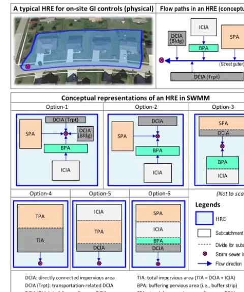
As mentioned earlier, an HRE can be modeled as a single subcatchment or multiple subcatchments in SWMM. In the SWMM model setup just described we used a single sub-catchment setup that was based on the results of an anal-ysis done with the goal of determining which among a se-ries of plausible HRE configuration options strikes a balance among the degree of spatial and hydrologic aggregation, out-put uncertainty, and comout-putational effort. The most spatially refined approach to a SWMM setup (Option 1 in this study as presented below) would be to discretize every piece of im-pervious and im-pervious surface as an independent subcatch-ment. This promises a decrease in model output uncertainty (Krebs et al., 2014; Sun et al., 2014), but requires specify-ing all the modelspecify-ing parameters and unique flow directions among all subcatchments, results in longer computational times, and produces data management burdens that are typi-cally not practical. The opposite extreme would be a highly generalized subcatchment characterization where the entire area is modeled as one subcatchment with just two subareas, lumping all the spatial heterogeneity into a fictional space that has no basis in physical reality. Within this continuum, we chose to consider six plausible options for representing urban spatial constructs that are constrained by the SWMM subcatchment/subarea paradigm were examined (Fig. 5). As shown in the legend of Fig. 5, each rectangle represents a subcatchment in SWMM, and the dotted line divides subar-eas within the subcatchment. A rectangle without a dotted line means the subcatchment consists of a single (homoge-neous) subarea, either 100 % impervious or pervious. The ar-rows represent flow routing directions. Conducting this as-sessment at the watershed scale would not only be tedious and time consuming to configure, but could be inappropri-ate because of potentially confounding effects introduced when the drainage network and groundwater algorithm are included in the simulation. We felt it more rational to base our assessment of HRE setup options at the scale of an HRE, i.e., the area that drains to a storm sewer inlet, and judge the results in comparison to the most spatially explicit option. Note, we do not have supporting observational data at this scale to prove this assumption. This would require flow data at the point of entry to a storm sewer inlet, which is very difficult to obtain in practice.

Instead, a hypothetical representation of a typical urban-scape was defined as the HRE and used to model eight syn-thetic single storm events for each of the six setup options (Fig. 5). The hypothetical HRE is meant to represent a typ-ical 4041 m2(1 acre) residential area consisting of 809.4 m2 (0.2 acre) DCIA, 1214.1 m2(0.3 acre) ICIA, and 2023.4 m2 (0.5 acre) PA. The DCIA consists of 607.0 m2 (0.15 acre)

DCIA: directly connected impervious area TIA: total impervious area (TIA = DCIA + ICIA)

DCIA (Trpt): transportation-related DCIA BPA: buffering pervious area (i.e., buffer strip)

DCIA (Bldg): building rooftops as DCIA SPA: standalone pervious area (i.e., non-BPA)

ICIA: indirectly connected impervious area TPA: total pervious area (TPA = BPA + SPA)

A typical HRE for on-site GI controls (physical) Flow paths in an HRE (conceptual)

Conceptual representations of an HRE in SWMM

Option-1 Option-2 Option-3

Option-4 Option-5 Option-6

DCIA (Bldg) DCIA (Trpt)

BPA

ICIA SPA

DCIA

BPA

ICIA

SPA DCIA

BPA

ICIA SPA

TIA TPA

DCIA TPA ICIA

DCIA BPA ICIA SPA

(Not to scale) Legends

HRE

Subcatchment

Divide for subareas Storm sewer inlet Flow direction

DCIA (Bldg)

DCIA (Trpt) ICIA

BPA SPA

[image:7.612.308.548.67.354.2]

(Street gutter)

Figure 5. A conceptual representation of the hypothetical HRE (20 % DCIA, 30 % ICIA, 10 % BPA, and 40 % SPA) and the six op-tions considered for representing this area in the setup of a SWMM model.

transportation-related surfaces (e.g., streets, driveways) and 202.3 m2(0.05 acre) building rooftops. The runoff from ICIA discharges through 404.7 m2(0.1 acre) BPA, thus the SPA of the area is 1618.7 m2(0.4 acre).

(8)

oppo-Table 1.Initial and calibrated modeling parameters for the Shayler Crossing watershed. “n/a” indicates the parameter is not applicable to the land cover type.

Land cover Length (m) Slope (%) n DS (mm) Ksat(mm h−1)

Initial Calibrated Initial Calibrated Initial Calibrated Initial Calibrated Initial Calibrated

Main building 9.1 7.6 10 15 0.014 0.01 2.0 1.3 n/a n/a

Misc. building 4.6 4.6 10 15 0.014 0.01 2.0 1.3 n/a n/a

Street 3.0 3.0 2 2.5 0.011 0.01 2.5 1.3 n/a n/a

Driveway 4.6 3.7 2 1.5 0.012 0.01 2.5 1.3 n/a n/a

Parking 3.0 3.0 1 1.5 0.012 0.01 3.0 1.3 n/a n/a

Sidewalk 0.9 0.9 1 1.5 0.012 0.01 3.0 1.3 n/a n/a

Other impervious 3.0 2.4 1 1.5 0.012 0.01 3.0 1.3 n/a n/a

Lawn 24.4 24.4 2 2 0.2 0.3 5.1 5.1 1.6 0.89

Forest 24.4 24.4 3 2 0.6 0.6 10.2 7.6 1.6 1.52

Agriculture 30.5 30.5 2 2 0.3 0.3 7.6 5.1 1.6 1.02

site (Rossman, 2015). Percent routed should be specified as 100 for both subcatchments. In options 4 through 6, the ar-eas are further aggregated to a single subcatchment represen-tation for an HRE in SWMM. Option 4 configures the sin-gle subcatchment with only two subareas, impervious and pervious areas. The runoff from pervious area discharges through impervious area (i.e., TIA=DCIA). In Option 5, DCIA and ICIA are independently modeled by specifying the subarea routing option as pervious and the percent routed as the ratio of ICIA/TIA. This option may be considered an unrealistic “green” development condition where runoff from ICIA is evenly distributed throughout the entire pervi-ous area, which means the entire pervipervi-ous area works like a buffer (i.e., TPA=BPA). Finally, in Option 6, LID con-trols in SWMM are used for modeling BPA and ICIA. BPA is modeled as a vegetated swale with a very small berm height, 2.54 mm (0.1 inch). In the “LID Usage Editor”, the “area of each unit” specifies the size of BPA and the “% of impervious area treated” is the fraction ICIA/TIA. With this configura-tion, the four hydrologically homogenous subareas – DCIA, ICIA, BPA, and SPA – are accounted for.

Lengths for overland flow (or sheet flow) were assumed to be 4.57 m (15 feet), 9.14 m (30 feet), 12.19 m (40 feet), and 15.24 m (50 feet) for transportation-related DCIA, build-ing rooftops as DCIA, ICIA, and pervious area, respectively. The surface slopes of these were assumed to be 3, 11, 5, and 2 %, respectively. Surface dimensions and slopes of typ-ical urban land cover components are based on construction codes or were inferred based on the GIS. The values selected are meant to represent typical residential areas in the United States. For example, the assumed values were derived us-ing overland flow from the center of the street to the curb in a crowned 9.14 m (30 feet) wide neighborhood street with 3 % cross-sectional slope for the crown, 18.29 m (60 feet) wide gable houses with 11 % cross-sectional slope for the rooftops, and pervious surfaces with 2 % slope on average. Every IA is modeled with 0.01 for Manning’s roughness

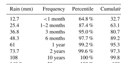
co-Table 2.Profile of the selected eight 24 h single storm statistics.

Rain (mm) Frequency Percentile Cumulative

12.7 <1 month 64.8 % 32.7 %

25.4 1–2 months 87.4 % 63.1 %

36.8 3 months 95.0 % 80.7 %

48.3 6 months 97.7 % 89.2 %

61 1 year 99.2 % 95.3 %

73.7 2 years 99.6 % 97.3 %

108 10 years 100 % 99.8 %

149.8 50 years 100 % 100 %

The percentile and cumulative percentage-based statistics qualify the exceedance probability of each event and the relative contribution of events of similar size or lower to the annual rainfall, respectively.

efficient (n)and 2.54 mm (0.1 inch) for depression storage (DS). Pervious area is modeled with 0.1 fornand 5.08 mm (0.2 inch) for DS. Identical infiltration parameters were ap-plied to all the options. In this hypothetical HRE model setup analysis, all of the six options were arranged using the same spatial and hydrologic characteristics. However, the ways DCIA, ICIA, BPA, and SPA were parameterized in SWMM were different among the options (Fig. 5).

[image:8.612.53.543.96.247.2] [image:8.612.323.533.293.403.2]

(9)

For example, the 90th percentile rainfall event is defined as the measured precipitation depth accumulated over a 24 h period for the period of record that ranks as the 90th per-centile rainfall depth based on the range of all daily event occurrences during this period. Values in the cumulative col-umn of Table 2 represent the percentage of annual cumula-tive precipitation depth, which are less than or equal to the specific rainfall depth during a 24 h period. In SWMM, the selected storms were distributed with 5 min intervals by ap-plying the Natural Resources Conservation Service (NRCS) Type-II distribution (USDA, 1986).

2.6 Calibration of the SHC watershed SWMM model Stream flows were measured at the outlet from a rating curve using water depth recorded at 10 min intervals. A tipping bucket rain gauge measured rainfall depths at 10 min inter-vals, with a minimum detectable rainfall depth of 0.254 mm (0.01 inch). The SWMM model for SHC (Fig. 6) was run for a 6-month period (1 April 2009 to 31 August 2009) where the first 4 months of this period were used to stabi-lize the continuous simulation, in particular for the ground-water simulation. This is defined as the model warm-up pe-riod, which is the time period required to achieve a stable condition wherein the groundwater level ceases to increase or decrease by a specified initial parameter threshold value. After the warm-up period, the last 2 months, from July to August 2009, were used for model calibration. Model cali-bration was done manually by adjusting the initial values for the 10 land cover types and using the different sets of BPA (see Fig. 3). Changes were integrated one at a time into every subcatchment using the area-weighting approach in an Excel spreadsheet. The calibrated modeling parameters for individ-ual land cover types are given in Table 1 alongside their ini-tial values. An Excel worksheet was created with embedded lookup and averaging functions so that changes made to the original values in Table 1 or switches between BPA sets con-figured using the different buffer distances could be easily propagated to changes in the related parameter values used in the SWMM model using the SWMM Excel Editor function. With this approach, the calibration effort is evenly applied to the urban land cover types, which in turn are propagated to the parameterization of all subcatchments, instead of cali-brating parameters individually for each subcatchment. This methodology assumes that urban land cover components are generalizable and independent from scale even though the subcatchments themselves are not generalizable or easily scalable. Also, notable about this approach, the parameter calibration domain remains the same even if the total num-ber of subcatchments is increased and/or the size of water-shed area is increased. If a land cover type does not maintain a sufficient level of homogeneity across the watershed under study, we would need to divide the land cover into subcate-gories and use more than one set of parameters for the land cover type in each category. For example, the main building

can be divided into two subcategories that represent slanted rooftops and flat rooftops independently, and the lawn area can be divided into multiple subcategories based on different surface slopes and/or soil infiltration properties. This can be handled by spatial analysis in GIS by overlaying land use, topography, or soil property data with the land cover layer.

Sensitivity analysis was conducted for the modeling pa-rameters of width, slope,nand DS for IA,nand DS for PA,

Ksat, and the size of BPA. Each parameter was decreased and

increased 5, 10, and 20 %, respectively, one at a time, and in separate model runs. The sensitivity of each parameter was estimated as

Sensitivity=(1MR/MR)/(1p/p), (1)

where MR is the modeling result in units of flow volume from the SWMM run,1MR is the change in SWMM mod-eling result based on change in parameter value,pis the pa-rameter value, and1pis the change in parameter value. 2.7 Modeling GI scenarios

GI scenarios are added to the model using the land cover database, soils, storm sewer systems, and GIS techniques to derive relevant BPA and may require some field investiga-tion to ground-truth the opinvestiga-tions. The general workflow for GI modeling is presented in the bottom half of Fig. A1. Im-plementing GI can be achieved by adjusting the hydrologic properties of individual land cover components, such as con-verting lawn area to shrub or forest (Lee et al., 2005). This sort of GI implementation can reduce the volume, peak, and speed of surface runoff and be modeled by adjusting DS, slope,n, or overland flow length for the converted land cover component. The one scenario we examined was decreasing DCIA by disconnecting the directly connected rooftop down-spouts that directly route flow from the main buildings to the sewer system. This effectively reclassifies main buildings as ICIA. After the downspouts are disconnected, the PA that re-ceives stormwater runoff from the disconnected rooftop now works as additional BPA. To model this additional buffer-ing capacity, the size of BPA is re-estimated and the percent of IA routed to BPA is changed in SWMM. The increase in size of the BPA under this GI scenario was estimated again using the spatial analysis tools in ArcGIS by changing the buffering distance value from the calibrated baseline value of 0.61 m (2 feet) to 3.1 m (10 feet) around ICIA, including the disconnected main buildings. As a result, the modeled GI scenario includes two types model changes: one that reflects the downspout disconnection and another the buffering area extension.

(10)

[image:10.612.102.495.65.453.2]

Figure 6.Diagram of the developed SWMM model for the Shayler Crossing watershed.

therefore the computed value of the width parameter as repre-sented in SWMM should also change. The methodology we present here provides a systematic way of changing the width parameter in a rational and objective manner to account for the modeled GI scenario. Unfortunately, the suitability of this modeling approach cannot be determined until a high density of GI has been implemented at a watershed scale with before and after field observations.

2.8 Hydrograph separation

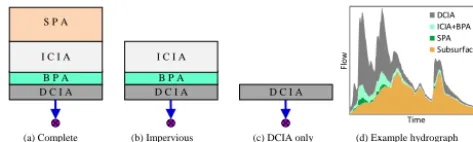
With the approach taken for the SWMM setup for both the baseline and GI scenario analysis adjustments can be made to apportion the simulated storm hydrologic loading from the watershed among the dominant sources: DCIA, ICIA+BPA, SPA, and subsurface flow. This can provide further insight into the effects of GI on watershed hydrology. For this pur-pose, the output from four SHC-SWMM runs were gener-ated:

– Run 1: every subcatchment is specified as described un-der Option 6 (as conceptually represented in Fig. 7a) with groundwater options parameterized to represent the base SWMM model.

– Run 2: groundwater options were excluded from the base model setup to remove any subsurface flow contri-butions to the stream flow hydrographs. The difference between (1) and (2) represents the stormwater contribu-tions to the stream as subsurface flow from the water-shed.

– Run 3: to estimate surface runoff from all impervious ar-eas (i.e., runoff from DCIA, plus ICIA through BPA) in the models without the groundwater, the SPA was also omitted from every subcatchment (Fig. 7b).

(11)

1 D C I A

(a) Complete (b) Impervious (c) DCIA only (d) Example hydrograph D C I A

B P A I C I A S P A

D C I A B P A I C I A

Fl

ow

[image:11.612.49.286.70.141.2]

Time DCIA ICIA+BPA SPA Subsurface

Figure 7.Conceptual representations of discrete SWMM models for hydrograph separation.

An example result of the hydrograph flow pathway sepa-ration is presented in Fig. 7d, and the process is summarized mathematically as follows:

Qtotal=QDCIA+QICIA+BPA+QSPA+Qsubsurface, (2)

Qsurface=QDCIA+QICIA+BPA+QSPA, (3)

Qsubsurface=Qtotal−Qsurface, (4)

QSPA=Qsurface−Qimperv, (5)

QICIA+BPA=Qimperv−QDCIA, (6)

where Qtotal is the total runoff with groundwater flow in

SWMM,Qsurfaceis the surface runoff without groundwater

flow,Qimpervis the runoff from impervious area (DCIA and

ICIA through BPA), QDCIA is the runoff from DCIA only, QICIA+BPA is the runoff from ICIA and BPA, QSPA is the

runoff from SPA only, andQsubsurface is the runoff through

groundwater flow (i.e., subsurface or lateral flow).

3 Results and discussion

The SHC watershed model parameter values pre- and post-calibration are presented in Table 1.

3.1 Spatial analysis

Table 3 reveals the results of the detailed spatial analysis con-ducted using the described GIS techniques. The fractional DCIA for buildings, streets, driveways, parking areas, and sidewalks are 96.1, 79.5, 94.2, 42.8, and 14.2 %, respectively. Overall, the study watershed is covered by 18.8 % DCIA, and three sets of BPA were derived for 0.30, 0.61, and 1.52 m buffer lengths. After calibration, the 0.61 m buffer around ICIA was selected for SHC. This means that the runoff from ICIA is discharged to the adjacent pervious area with 0.61 m buffer width, based on runoff volume and timing in hydro-graphs (see Figs. 10 and 11). This existing buffer covers 22 683.5 m2of the pervious area, which is 2.3 % of the entire watershed and 3.0 % of the pervious area. As the baseline, the SHC watershed consists of 18.8 % DCIA, 5.2 % ICIA, 2.3 % BPA, 73.1 % SPA, and 0.6 % water. Under the modeled GI scenario of disconnecting rooftop drains and extended BPA, the DCIA is reduced to 9.6 %, the ICIA increases to

14.4 %, the BPA increases to 17.2 %, and the SPA is reduced to 58.2 % of the total area, respectively.

3.2 The hypothetical HRE modeling analysis

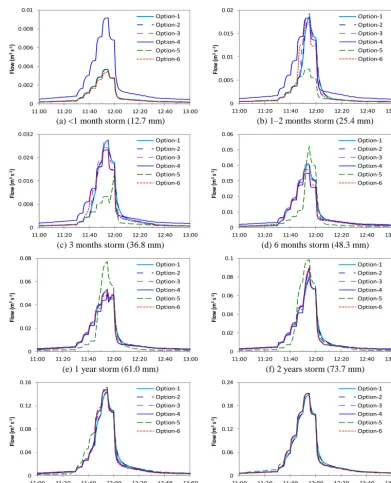
The eight single storm hypothetical HRE modeling analy-sis with the six discretization options resulted in 48 SWMM runs. As explained earlier, this was done to determine which HRE configuration option best balances model complexity and presumed accuracy. Each simulated storm was assumed to last from midnight to midnight. Results are presented as hydrographs between 11:00 and 13:00 where most con-centrated rainfall occurs in the NRCS Type-II distribution (USDA, 1986) (Fig. 8). In large storms, larger than a 5-year storm in particular, all six types of spatial discretization pro-duce very similar hydrographs as shown in Fig. 8g, h. The modeled flow rates and total runoff volumes are almost iden-tical.

In the large storm situation, all of the PAs are saturated in the early stage of the storm. Once saturated, the PAs are not able to provide any additional on-site hydrologic control and behave as IA. In view of this, any of the spatial discretization options would be suitable for analyzing flood controls and in designing a drainage system based on a 10-year storm. How-ever, this is not the relevant case for evaluating GI imple-mentation, which focuses on controlling smaller storms. For storms smaller than a 2-year event, considerable differences were found among the simulated hydrographs (Fig. 8a–e).

(12)

[image:12.612.129.467.85.295.2]

Table 3.Land cover status of Shayler Crossing watershed.

Surface components DCIA (m2) ICIA (m2) Sum (m2) Fraction

Impervious areas Building 91 770.0 3756.2 95 526.2 9.6 %

Street 57 610.5 14 897.2 72 507.7 7.3 %

Driveway 33 554.7 2083.7 35 638.4 3.6 %

Parking 2362.7 3154.1 5516.8 0.6 %

Sidewalk 1646.9 9990.3 11 637.2 1.2 %

Miscellaneous – 17 766.8 17 766.8 1.8 %

Sum of IA 186 944.7 51 648.4 238 593.1 24.0 %

Pervious areas Lawn 400 667.4 40.3 %

Agriculture 219 430.4 22.1 %

Forest 128 558.1 12.9 %

Sum of PA 748 655.9 75.4 %

Water Wet pond 5014.2 0.5 %

Swimming pool 998.9 0.1 %

Sum of water 6013.0 0.6 %

Sum 993 262.0 100 %

the entire pervious area works like BPA. The expanded on-site pervious buffer can thoroughly control runoff from ICIA until the DS and infiltration capacity of BPA are fully satu-rated. Once the hydrologic capacities for on-site controls are fully saturated, the entire PA hydrologically responds more or less like IA. Once a subcatchment DS fills and exceeds infiltration capacity, this unrealistic green development con-dition may result in higher peak discharges than the other options.

From the hypothetical modeling analysis, it can be sur-mised that an extensive on-site green infrastructure imple-mentation could result in more frequent local flooding, e.g., water intrusion into basements. This may be especially the case when evaluating scenarios for locations where medium-size storms have a long duration, like during the wet season of the Pacific Northwest of the United States. The compara-tively high runoff estimated for Option 5 (Fig. 8d–f) would be maintained until all PA is saturated by increased rainfall intensity. If a smaller portion of PA is modeled as BPA, while all the other conditions are kept the same, the BPA reaches the saturated condition under a smaller storm. Once the BPA is saturated the area hydrologically responds like IA. How-ever, SPA (i.e., non-buffering pervious area) can still control rainfall within the area. This analysis suggests that it is im-portant to properly define the area of BPA especially when analyzing GI alternatives for on-site stormwater controls, as we surmised originally. Therefore, Option 5 is not suitable for modeling a GI scenario because it ignores the actual sig-nificance of variance in BPA. It is a common modeling prac-tice in SWMM to treat all pervious area the same (as in op-tions 4 or 5 in Fig. 5), even though only the BPA can receive water from ICIA. As shown in Fig. 8, simulated runoff by

options 4 or 5 would presumably be inaccurate, especially for the<1-year small storms.

Figure 9 contains graphs comparing the results among the six options (Fig. 5), showing the relative difference for peak flow, average flow, and total runoff volume for each of the five other options compared to Option 1, presumably the most accurate one, in terms of output uncertainty because the level of spatial lumping is the lowest.

The relative differences reported in Fig. 9 (“variation from the result of 5-subs” in theyaxis) were estimated as (MRk_j−

(13)

(a) <1 month storm (12.7 mm) (b) 1–2 months storm (25.4 mm)

(c) 3 months storm (36.8 mm) (d) 6 months storm (48.3 mm)

(e) 1 year storm (61.0 mm) (f) 2 years storm (73.7 mm)

(g) 10 years storm (108.0 mm) (h) 50 years storm (149.8 mm)

0 0.002 0.004 0.006 0.008 0.01

11:00 11:20 11:40 12:00 12:20 12:40 13:00

Fl ow (m 3s -1) Option-1 Option-2 Option-3 Option-4 Option-5 Option-6 0 0.005 0.01 0.015 0.02

11:00 11:20 11:40 12:00 12:20 12:40 13:00

Fl ow (m 3s -1) Option-1 Option-2 Option-3 Option-4 Option-5 Option-6 0 0.01 0.02 0.03 0.04 0.05 0.06

11:00 11:20 11:40 12:00 12:20 12:40 13:00

Fl ow (m 3s -1) Option-1 Option-2 Option-3 Option-4 Option-5 Option-6 0 0.02 0.04 0.06 0.08 0.1

11:00 11:20 11:40 12:00 12:20 12:40 13:00

[image:13.612.99.490.71.554.2]

Fl ow (m 3s -1) Option-1 Option-2 Option-3 Option-4 Option-5 Option-6

Figure 8.Hypothetical HRE SWMM modeling results.

tion criteria, especially in terms of the level of effort required in model setup, configuring parameter values and output un-certainty.

3.3 SHC watershed-scale modeling results

Option 6 (Fig. 5) was used to set up the SWMM model for the SHC watershed as described above. The SHC model consists of 191 subcatchments and 269 junctions and

(14)

(a) Average flow rate

(b) Peak flow rate

(c) Total runoff volume -100 % -50 % 0 % 50 % 100 % 150 %

12.7-mm 25.4-mm 36.8-mm 48.3-mm 61.0-mm 73.7-mm 108.0-mm 149.8-mm

V ar ia ti o n fr o m t h e re su lt o f 5 -su b s

24 h synthetic storms

Option-1 Option-2

Option-3 Option-4

Option-5 Option-6

V ar ia ti o n fr o m t h e re su lt o f 5 -s u b s

Option-1 Option-2

Option-3 Option-4

Option-5 Option-6

V ar ia ti o n fr o m t h e re su lt o f 5 -s u b s

[image:14.612.314.540.69.167.2]

Option-1 Option-2 Option-3 Option-4 Option-5 Option-6 -100 % -50 % 0 % 50 % 100 % 150 % -100 % -50 % 0 % 50 % 100 % 150 %

Figure 9.Comparison of the hypothetical HRE modeling results.

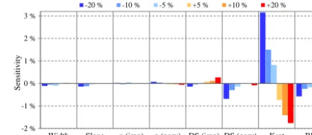
(48.3 mm d−1) based on the storm statistics for the study area (see Table 2). While the 3 % change in total runoff is not sig-nificant in sensitivity, the most sensitive parameter wasKsat,

followed by BPA and DS. Whereas the changes inKsataffect

the entire PA (75.4 % of SHC), the changes in BPA affect a much smaller area (2.3 % of SHC for the baseline condition) than PA. The other parameters (i.e., width, slope, and n) were found not to be as sensitive, with negligible changes in results

≤ ±0.15 % even for±20 % change in the individual param-eter value. When land cover status is represented accurately in a SWMM model, certain parameters will be less sensi-tive because of the underlying hydraulic and spatial realities are well represented. For example, the parameters represent-ing the impervious land cover types in this modelrepresent-ing analysis were found to be less sensitive than pervious area parameters. Model calibration was conducted by adjusting the land-cover-based modeling parameters and BPA to the entire

1 -2 % -1 % 0 % 1 % 2 % 3 %

Width Slope n (imp) n (perv) DS (imp) DS (perv) Ksat BPA

S

ensit

ivi

ty

-20 % -10 % -5 % +5 % +10 % +20 %

Figure 10.Sensitivity analysis of the SWMM parameters at SHC.

1 0 100 200 0 1 2 3

1-Jul 7-Jul 13-Jul 19-Jul 25-Jul 31-Jul 6-Aug 12-Aug 18-Aug 24-Aug 30-Aug

R a in fa ll (m m h -1) F lo w ra te ( m 3s -1)

Observed flow Modeled flow Rainfall

[image:14.612.53.278.70.468.2]

Nash-Sutcliffe coeff. = 0.852 R2= 0.871

Figure 11.Watershed-scale SWMM modeling results from 1 July 2009 to 31 August 2009.

study watershed. As shown in Table 1, parameters for the impervious land cover types changed little and were made equivalent fornand DS. As expected, parameters for the per-vious land cover types needed more adjustment than those for the impervious. The initial value ofKsat was defined using

the site-specific soil types (mainly silty loam clay), but the values for the individual pervious land cover types were var-ied by the model calibration effort. WhereasKsatfor forest

area was adjusted only slightly (i.e., 1.6 initially to 1.52 for the final calibration), the values for lawn (or landscaped area) and agriculture required more adjustment (from 1.6 initial to 1.02 for agriculture, and from 1.6 initial to 0.89 for lawns). The relatively large changes forKsatare indicative of more

soil compaction for urban and agricultural soils compared to the expected native soil condition.

The measured rainfall intensities and stream flow rates, along with the calibrated model results are presented in Fig. 11. The modeled hydrographs are well matched with the measured data at the watershed scale with a Nash–Sutcliffe coefficient=0.852 andR2=0.871.

[image:14.612.310.544.210.301.2]

(15)

(a) Land cover components (b) Hydrologic components 18.8 %

9.6 %

2.3 % _{17.2 %}

5.2 %

14.4 % 73.1 %

58.2 %

0.6 % 0.6 %

Baseline GI

DCIA BPA ICIA SPA Water

19.1 %

10.5 % 28.5 %

36.2 %

43.8 % 43.4 %

8.6 % 9.9 %

Baseline GI

[image:15.612.51.284.68.222.2]

DCIA Others Subsurface Loss

Figure 12. Relative percentages of(a)land cover and(b) hydro-logic components computed for the period 1 July 2009 to 31 August

2009. In(b)“others” represents surface runoff from areas other than

DCIA, “subsurface flow” is the subsurface contribution, and “loss” is rainfall loss by evaporation or deep percolation.

(a) Baseline condition

(b) GI implementation scenario

0.00 0.07 0.14 0.21 0.28 0.35

0:00 6:00 12:00 18:00 0:00 6:00 12:00 18:00 0:00 6:00 12:00 18:00 0:00

F

low

(

m

3s -1)

Time (22 to 24 July 2009)

Subsurface Others DCIA

Total volume

40.3 %

13.0 % 46.7

%

0.00 0.07 0.14 0.21 0.28 0.35

0:00 6:00 12:00 18:00 0:00 6:00 12:00 18:00 0:00 6:00 12:00 18:00 0:00

F

low

(

m

3s -1)

Time (22 to 24 July 2009)

Subsurface Others DCIA

Total volume

42.4 %

28.7 % 28.9

%

Figure 13.Hydrograph separation and volumetric percentages con-tributing to stream flow for the period 22 to 24 July 2009.

slightly higher in the GI scenario, but that the duration of flows slightly smaller than this peak is longer in the baseline scenario.

While the results from applying the hydrograph separation cannot be validated without extensive field measurements, the exercise provides insight to the potential effectiveness and rationale for developing strategies for GI in the water-shed. For instance, about 48 % of the volumetric stream flow was contributed through subsurface flow over the simulation

period, even though the study watershed is characterized with poorly infiltrating soils. After applying the GI scenario, al-though the subsurface flow contributed a similar fraction to the stream flow, the fractional contributions of surface runoff from DCIA and the other areas are significantly changed (Figs. 12b and 13). This situation arises not from a change in land cover but the internal flow paths taken by the runoff. The result is reduced runoff from DCIA but increased runoff from the other areas (i.e., ICIA, BPA, and SPA).

From a water quality management perspective, it is neces-sary to consider hydrologic and contaminant discharge pro-cesses with respect to their sources and transport pathways. For example, if the watershed has water quality issues related to nutrients, the management effort might pay more atten-tion to the stormwater discharge from pervious areas that in-clude fertilizer applications. If GI were designed to intercept runoff from DCIA in the watershed, an unintended conse-quence could result from increased runoff volume traveling through a pervious area with elevated standing stocks of sol-uble or erodible nutrients. In this case, it would be important to consider turf management practices.

Another example of how the hydrograph separation ap-proach (Fig. 13) provides additional opportunities for inter-preting hydrodynamics before and after applying the GI sce-nario is revealed by considering that disconnecting down-spouts reduced the total runoff volume, but also resulted in a higher peak flow (note the 16:00 time point on 22 July 2009 in Fig. 13). This result is like the single storm analysis using Option 5 (Fig. 5). Overall the flow volume is reduced from the GI scenario. However, when the peak occurred around 15:30 (shown in Fig. 13), the capacity of the GI for ling stormwater was already exceeded because of control-ling runoff during the previous rainfall that occurred between 7:00 and 14:00. Under this saturated condition, even the di-rect rainfall to the GI area will be discharged with minimum abatement. If there is no GI (as in the baseline condition), the same area receives only direct rainfall, there is no additional runoff from the impervious area, and that rainfall is con-trolled by still-available surface depression storage and not-saturated infiltration capacity. In the 22 July 2009 situation, the stormwater control capacity (mainly DS and infiltration) of the extended BPA is saturated by earlier rainfall. Once saturated, the BPA discharges higher runoff. The modeled GI contributes much higher runoff volume from PA, which might be nutrient enriched. With the hydrograph separation analysis, we gain insight to the consideration of stormwater management objectives and extend the utility of SWMM.

4 Summary and conclusions

[image:15.612.52.282.310.552.2]

(16)

discretization approach for GI modeling was initially veri-fied with a hypothetical urbanscape analysis using eight syn-thetic storms of various sizes. We evaluated our approach to SWMM subcatchment parameterization using the hypothet-ical analysis that allowed for the qualification of five differ-ent options relative to one that would be considered the most spatially explicit and, therefore, result in the least amount of output uncertainty (see Fig. 9). From the hypothetical analy-sis, the best option was selected to develop a watershed-scale SWMM model at the study area. The simulated hydrographs by the developed watershed-scale SWMM model were well matched with observed data over a 2-month continuous sim-ulation (Nash–Sutcliffe coefficient=0.852;R2=0.871) af-ter minimal calibration effort. A GI scenario that modeled downspout disconnection from all the main buildings that are DCIA was described. We demonstrate how simple model ad-justments can be made to separate the total and surface runoff among primary pathways that runoff takes before discharg-ing to the natural stream network. This hydrograph separa-tion procedure can shed light on GI design requirements and water quality management.

The optimal spatial discretization scheme distinguishes DCIA from ICIA, and BPA from SPA, and explicitly models these as subareas within each subcatchment parameterization in SWMM. This approach is particularly useful when mod-eling the impact of small storms, i.e., when BPA can control all or most of ICIA runoff. The land-cover-based spatial dis-cretization approach is scale-independent, can be applied di-rectly to a larger watershed as long as any heterogeneity in landscape properties is accounted for in the GIS setup (e.g., by dividing land cover components into multiple subgroups such as flat and slanted rooftops, high and low sloped ur-ban hillslopes, or B and C type hydrologic soil types), and affords the opportunity to evaluate urban stormwater man-agement strategies with presumably decreased output uncer-tainty for small storms and expanded applicability to GI plan-ning, design, and implementation. Parameters are adjusted per SWMM subcatchment in a typical calibration approach, which is scale-dependent and requires more effort in larger watersheds. In our approach, a SWMM model is calibrated by adjusting parameters per land cover component, which are categorized by urban development codes or general construc-tion specificaconstruc-tions for land uses. Overall this study demon-strates the relative effectiveness of different approaches in drainage area characterization using highly resolved spatial data to the setup and analysis of a SWMM model that should improve its utility for simulation of GI.

Data availability. The data will be accessible via the US EPA’s

Environmental Dataset Gateway (https://edg.epa.gov/metadata/ catalog/main/home.page).

Competing interests. The authors declare that they have no conflict

of interest.

Disclaimer. The US Environmental Protection Agency, through its

(17)

Appendix A: Miscellaneous procedures for SWMM modeling for GI analysis

For a full description of the steps used to set up a SWMM model for GI analysis using the methods outlined here see Lee et al. (2017), which is available for free download from the USEPA at https://nepis.epa.gov/Exe/ZyPDF.cgi/ P100TJ39.PDF?Dockey=P100TJ39.PDF, (last access: 20 April 2018). The procedure for developing the baseline model is schematically diagrammed in Fig. A1. To reduce model complexity, the original 16 land cover types (men-tioned in Sect. 2.2.2) were reduced to 10 by merging the paved walking paths, patios, and miscellaneous impervi-ous areas with other imperviimpervi-ous areas; the dry ponds were merged with lawn areas; the detention area was merged with forest; and the surface areas for wet ponds and pools were modeled as IA without DS. The structures of the dry ponds, detention areas, and wet ponds were modeled as SWMM storage units. The final 10 land cover classifications include main buildings, miscellaneous buildings, streets, driveways, parking, sidewalks, other impervious areas, lawn, forest, and agriculture.

A1 Determining values for SWMM subcatchment parameters: area-weighting approach

Unique values for representing the corresponding area, width, slope, imperviousness,n, DS, and infiltration param-eters (Ksat, Suct, and IMD for the Green–Ampt option) were

defined per SWMM subcatchment using GIS and a spread-sheet.

The area of each land cover type within a subcatchment was estimated using ArcGIS. The SWMM parameter “char-acteristic width” was estimated using an area-weighted flow length, as recommended in the SWMM Applications Manual (Gironás et al., 2009). This manual suggests, “If the over-land flow length varies greatly within the subcatchment, then an area-weighted average should be used.” Comparatively, in conventional SWMM modeling, the characteristic width is computed by dividing the subcatchment area by the av-erage maximum overland flow length. Then adjustments are made to the characteristic width during model calibration to produce the best fit to the measured runoff hydrographs. The following area-weighting calculation describes how the char-acteristic width for a SWMM subcatchment was estimated in this study, whereirepresents all the individual land cover types within the subcatchment:

Length=6(Length_iAreai)/6(Areai), (A1)

Width=6(Areai)/Length. (A2)

Other parameters were also defined as area-weighted aver-ages per subcatchment (e.g., slope and infiltration parame-ters) or subarea (e.g., n and DS). This area-weighting step is used following the typical approach recommended to ac-count for the spatial lumping that effectively averages patchy

land cover types within SWMM subcatchments (Gironás et al., 2009; Rossman and Huber, 2016). Hence, the extent of each individual type of land cover in a subcatchment is used to area-weight the assigned parameter values. For example, if IA within a subcatchment consists of two building rooftops, two driveways, and one section of street, the associated IA in SWMM is assigned values for DS based on an area-weighted average using the corresponding nominal values presented in Table 1, DSimp=6(DSiAi)/6(Ai), where DSimpis the

as-signed DS for the impervious subarea within the subcatch-ment,Ais the size of an individual impervious land cover type within the subcatchment, and i is an individual land cover type. Calculations for area-weighting were all done in a Microsoft Excel spreadsheet that was configured for di-rect copy and pasting as the SWMM input file using the EPA–SWMM Excel Editor function (see Lee et al., 2017, for specifics and Fig. A1). Two sets ofnand DS were defined per SWMM subcatchment – one set for the impervious sub-area and the other for the pervious subsub-area. Where available, relevant values were obtained from experience in the water-shed or using GIS (e.g., overland flow length), or as sug-gested by the SWMM manual (Huber and Dickinson, 1988; Rossman, 2015). The SHC watershed has silty loamy clay soils throughout. Based on this soil type, Suct was set to be 165 mm using the SWMM User’s Manual (Rossman, 2015). IMD was modeled using the default value (0.22) in the EPA-SWMM. The actual IMD is dynamically updated at every modeling time step. The developed SWMM model runs for a 6-month period where the first 4 months of this period are used to stabilize the continuous simulation (i.e., the warm-up period). Hence, the IMD value when modeling results are first reported may not reflect the initial value assigned during model setup. The values forKsat were amended during the

model calibration to comprise surface compaction in lawn, agricultural, and forest areas (Horton et al., 1994; Gregory et al., 2006). However, we did not try to change the values of Suct and IMD during the calibration. Although the status and spatial extent of each land cover type within each HRE are different, the parameter values were assigned indepen-dent of the HRE in which it resided (Table 1). This parameter assignment methodology at the level of land cover compo-nents reduces model complexity by minimizing the amount of subcatchment-specific parameterizations that may need to be considered during calibration.

A2 Setting up the BPA

(18)

G I S

Spreadsheet

SWMM

Baseline condition

Acceptable? No

Yes Baseline model, modeling results Baseline modeling

Observed data Attribute data

Spatial data

Model calibration

Spatial analysis

LC components Spatial overlay

Delineate HREs

Topography Storm sewer systems

HREs-components

G I S

A r c G I S Data

collection

Parameters per component

Area-weighting

Spreadsheet

M S – E X C E L

Components per HRE

Estimated parameters

for HREs GIS-SWMM

interface

S W M M

PCSWMM EPA-SWMM Stormwater simulation

G I S

Spreadsheet

SWMM Satisfied?

No Yes GI requirements

GI model(s), modeling results GI scenario(s)

Modeling for GI implementation

Attribute data

Spatial data

[image:18.612.49.285.66.305.2]

Scenario simulation

Figure A1.Procedures for SWMM modeling for GI analysis. LC stands for land cover. Conceptual workflow for each of the colored

boxes is given in the middle of the diagram. Symbols ( )

are used to label workflow connections within the colored boxes. Top panel depicts the general steps used for baseline model setup, while the bottom panel adds GI considerations. “Acceptable?” indi-cates whether the statistical significance between the modeled and

the observed hydrographs (e.g., Nash–Sutcliffe coefficient orR2)is

acceptable. “Satisfied?” indicates whether the modeling results are satisfied with the GI requirements.

width was set to 18.3 m (60 feet), was equal across all sub-catchments, and was based on the average linear footage of BPA around the existing ICIA from distance measurements made using the GIS on a number of common ICIA features in the watershed, e.g., driveways, sidewalks, and miscella-neous outbuildings. Individual BPAs within a subcatchment are assumed to be parallelly aggregated in setting up the veg-etated swale. The initial saturation was also equal across all subcatchments – set at 25 % (this value self-equilibrates after the model warm-up period, see Sect. 2.6). The berm height of the vegetated swale was set at 2.54 mm (0.1 inch) to mini-mize any storage effect within the berm, which is the case for real BPA, and vegetation volume fraction was set to be 0. The percentage of subcatchment imperviousness contributing to the BPA (i.e., the ICIA) is obtained by dividing the ICIA by the total IA. Since the total pervious area remains identical for each HRE, the sizes of SPA for individual HREs can be determined as SPA=TPA – BPA for the three different sizes of BPA, which were derived by applying three different dis-tances for the proximity analysis in GIS. When we calibrated the model, we checked which one, among the three cases of

BPA sizes established above, would calibrate the best for var-ious storm sizes.

A3 The groundwater component

In SWMM groundwater flow is estimated by the following equation (Rossman, 2015):

Qgw=A1(Hgw−H∗)B1−A2 Hsw−H∗B2 (A3)

+A3HgwHsw,

whereQgwis the groundwater flow rate [L3T−1];Hgwis the

height of saturated zone above the bottom of aquifer [L];Hsw

is the height of surface water above the bottom of the aquifer [L];H∗is the threshold groundwater height [L]; andA1,A2, A3,B1, andB2is the empirically derived coefficients.

The top of the saturated zone is placed somewhere be-tween the soil surface and the bottom of the aquifer. The

H∗is identical to the height of the streambed above the bot-tom of the aquifer (Rossman, 2015). No measurement data were available for relative elevations of the saturated zone or the bottom of the aquifer for the study area, but even with these values the groundwater parameterization in SWMM cannot be explicitly configured given the five coefficients that need specification (Eq. A3). Therefore, as is typical, we based the groundwater simulation on the elevation differ-ence between individual subcatchment surface and its nearest stream bottom, which affectsHgw. Groundwater modeling

(19)

List of abbreviations

A1,A2, andA3 Empirically derived coefficients

ASCE American Society of Civil Engineers

B1andB2 Empirically derived coefficients

Bldg Building

BPA Buffering pervious area that receives and controls runoff from impervious area DCIA Directly connected impervious area

DS Depression storage

DS_imp Depression storage for impervious area ESRI Environmental Systems Research Institute

GI Green infrastructure

GIS Geographic Information System

H∗ Threshold groundwater height