1Global Institute for Water Security, University of Saskatchewan, National Hydrology Research Centre, Environment Canada,
11 Innovation Boulevard, Saskatoon, SK, S7N 2H5, Canada
2National Hydrology Research Centre, Environment Canada, 11 Innovation Boulevard, Saskatoon, SK, S7N 3H5, Canada 3Departamento del Agua, Centro Universitario Regional Litoral Norte, Universidad de la República, Salto, Uruguay
Correspondence:Fuad Yassin ([email protected])
Received: 4 January 2019 – Discussion started: 16 January 2019
Revised: 30 July 2019 – Accepted: 12 August 2019 – Published: 17 September 2019
Abstract. Reservoirs significantly affect flow regimes in watershed systems by changing the magnitude and timing of streamflows. Failure to represent these effects limits the performance of hydrological and land-surface models (H-LSMs) in the many highly regulated basins across the globe and limits the applicability of such models to investigate the futures of watershed systems through scenario analysis (e.g., scenarios of climate, land use, or reservoir regulation changes). An adequate representation of reservoirs and their operation in an H-LSM is therefore essential for a realis-tic representation of the downstream flow regime. In this paper, we present a general parametric reservoir operation model based on piecewise-linear relationships between voir storage, inflow, and release to approximate actual reser-voir operations. For the identification of the model ters, we propose two strategies: (a) a “generalized” parame-terization that requires a relatively limited amount of data and (b) direct calibration via multi-objective optimization when more data on historical storage and release are available. We use data from 37 reservoir case studies located in sev-eral regions across the globe for developing and testing the model. We further build this reservoir operation model into the MESH (Modélisation Environmentale-Surface et Hy-drologie) modeling system, which is a large-scale H-LSM. Our results across the case studies show that the proposed reservoir model with both parameter-identification strategies leads to improved simulation accuracy compared with the other widely used approaches for reservoir operation simu-lation. We further show the significance of enabling MESH with this reservoir model and discuss the interdependent
ef-fects of the simulation accuracy of natural processes and that of reservoir operations on the overall model performance. The reservoir operation model is generic and can be inte-grated into any H-LSM.
1 Introduction
1.1 Background and motivation
Despite the benefits in terms of enhancing water avail-ability in support of food security, power supply, etc., dams result in several negative environmental and social conse-quences. Adverse environmental effects include changes in natural river dynamics in terms of water temperature, sedi-ment and nutrient transport, etc., and the fragsedi-mentation and loss of biodiversity (Vörösmarty et al., 2010). Reservoirs can also intensify evaporation by increasing the surface area of water exposed to direct sunlight and air and through water supply for irrigation (de Rosnay, 2003; Pokhrel et al., 2012). Other environmental impacts of dams include the alteration of landscape due to dam construction and changes to land– atmosphere interaction that can have a profound impact on local and regional climate (Hossain et al., 2012; Degu et al., 2011). Adverse social effects include the displacement of people living near the dam site, changes to fishing patterns, and downstream erosion (Strobl and Strobl, 2011, p. 449). There are research gaps remaining in evaluating both posi-tive and negaposi-tive social impacts of dams (Kirchherr et al., 2016). Such gaps have been the subject of many studies in both academia and industry for years and, recently, have led to the formalization of the study area of “socio-hydrology” (Sivapalan et al., 2012; Sivakumar, 2012).
Dams and reservoirs change the natural flow regimes in rivers both in terms of magnitude and timing of flows. As a result, for rivers that contain large or small dams and reser-voirs, flow regimes are a combination of natural and managed flows. Various modeling communities manage this mix of natural and managed flows differently. Archfield et al. (2015) compare three families of models that can be used at con-tinental scales: catchment models (CMs), global water se-curity models (GWSMs), and land-surface models (LSMs). CMs generally ignore water management and focus on un-managed headwater catchments. GWSMs have been utilized in global-scale streamflow simulations and generally focus on large-scale water management issues, which are hindered by a lack of data on large-scale water management and opera-tional decisions. LSMs have tradiopera-tionally focused on provid-ing lower boundary conditions for atmospheric models but are increasingly being used for hydrological applications in which they are referred to as hydrologic land-surface mod-els (H-LSMs). LSMs generally ignore water management (Clark et al., 2015; Davison et al., 2016), with a few excep-tions (e.g., Voisin et al., 2013a, b). A fourth family of water models, which is relevant to the work presented here, are wa-ter management models (WMMs; Labadie, 1995; Yates et al., 2005). Water modelers who know how the water is managed within their basins of interest generally use WMMs (Lund and Guzman, 1999; Labadie, 2004; Kasprzyk et al., 2013). These models contain very detailed representations of water management decisions but often consider natural flow pro-cesses in a much more rudimentary fashion than CMs.
Modeling the many managed basins around the world us-ing the current generation of CMs or LSMs can result in models with limited fidelity, questions the credibility of their predictions of future water resources in basins with dams and reservoirs. Therefore, there is a pressing need for bet-ter characbet-terization and integration of the operation of dams and reservoirs into hydrological modeling frameworks us-ing CMs and LSMs (Nazemi and Wheater, 2015a, b; Pokhrel et al., 2016; Wada et al., 2017). This need motivated the ob-jectives of this study, described in Sect. 1.2, and some previ-ous research, outlined in Sect. 2. The integration of reservoir regulation into hydrological modeling frameworks will im-prove our ability to simulate highly regulated basins around the globe, leading to better understanding of historical con-ditions of water resource systems and improved assessment and prediction of their future vulnerability to climate and en-vironmental change.
1.2 Objectives
Building upon previous research, this study aims to do the following:
– Develop and test an improved reservoir operation model that can be integrated into any CM and LSM at any scale but in particular at large scales. Of interest is a simple but effective parameterization that can be ad-justed to varying levels of data availability.
– Integrate the developed reservoir operation model into an LSM and evaluate its performance when working in combination of other processes in the model. Also of in-terest is assessing the potential conceptual and technical issues in this integration.
Another potentially very fruitful but largely unexplored ap-proach would be to couple CMs and LSMs with WMMs, but that approach is not examined here due to the fact that WMMs generally require extensive information on how wa-ter is managed within a basin, whereas we are particularly interested in the more generic case when this information is likely to be limited or unavailable.
Chang et al., 2010; Fraternali et al., 2012; Razavi et al., 2012; Asadzadeh et al., 2014; Guo et al., 2013), a gap still exists between the methodologies applied for local- and regional-scale reservoir operations and management and the repre-sentation of reservoir operation in Earth system models, par-ticularly in LSMs. This gap is due to a twofold challenge. First, the upscaling of methodologies used at smaller scales to larger scales is non-trivial; second, the availability of data on reservoir operation and water use is often limited in many parts of the world. For example, the reservoir purpose and op-erational details are not always known, and large reservoirs typically serve several purposes (Wisser et al., 2010). As a re-sult, most current hydrological modeling activities with CMs and LSMs, if not all, offer only a limited capability in sim-ulating reservoir operations, whereas reservoir operation in practice involves a complex set of human-driven processes and decisions.
The existing reservoir operation methods in hydrologic models can be categorized roughly into three groups based on their level of complexity in representing flow regula-tion: (1) natural lake methods, (2) inflow- and demand-based methods, (3) artificial neural-network (NN) techniques, and (4) target storage-and-release-based methods.
2.1 Natural lake methods
The most primitive methods use formulations developed for the simulation of natural lakes or uncontrolled reservoirs. In these methods, the downstream release is calculated as a function of reservoir storage characterized by some empirical parameters (Meigh et al., 1999; Döll et al., 2003; Pietroniro et al., 2007; Rost et al., 2008). For instance, Meigh et al. (1999) calculate the release byQt=St1.5, whereQt andSt are re-lease and reservoir storage, respectively. Their method was later modified by Döll et al. (2003) such thatQt=b1(St− Smin)
St−Smin Smax−Smin
b2
, whereb1andb2are release coefficients,
and Smin and Smax are minimum and maximum allowable
reservoir storages. The advantage of this method, as shown in Döll et al. (2003), is its minimal data requirement, which supports its global applicability to model lakes, reservoirs, and wetlands. However, it has limited functionality in
ade-method used in Wisser et al. (2010); it estimates the release as a function of mean annual inflow and a set of empirical pa-rameters that can be calibrated in the absence of information on the actual operation of a reservoir.
Hanasaki et al. (2006) pioneered the development of in-flow and demand reservoir models and laid the foundation for many subsequent developments. The method of Hanasaki et al. (2006) simulates reservoir release at a monthly time step within a global routing model and accounts for wa-ter withdrawals for reservoirs categorized as irrigation reser-voirs. They grouped reservoirs serving all other purposes as non-irrigation reservoirs. This approach first estimates a pro-visional total annual release at the beginning of the water year based on the long-term mean annual inflow adjusted by an annual release coefficient. Then, a monthly provi-sional release is estimated based on the purpose of the reser-voir (irrigation or non-irrigation). Downstream demands are accounted for in irrigation reservoirs only. The provisional monthly release for large reservoirs is then modified by the annual release coefficient to calculate the actual monthly re-lease, and the provisional monthly release for small reser-voirs is additionally adjusted based on the monthly inflow to calculate the actual monthly release. The release coeffi-cient is estimated as a function of the reservoir storage at the beginning of the operational year and the reservoir capacity (the formulation of Hanasaki et al., 2006, is briefly explained in Sect. 3.4). The release coefficient reduces the current year release if the storage at the beginning is low and vice versa. Thus, the release coefficient accounts for inter-annual vari-ability and facilitates the representation of strategies to over-come reservoir depletion in dry years and flood overtopping in wet years.
(which is not known yet) could be high, and vice versa. Addi-tionally the simplification of complex reservoir operation in Hanasaki et al. (2006) by using the mean annual inflow and a release-constraining coefficient produces errors. However, the method is generic and has low data requirements, which are advantageous. The results showed that the reservoir algo-rithm improved monthly discharge simulation compared to the natural lake method (Hanasaki et al., 2006). The approach is effective and has found wide applicability in several global hydrological and land-surface models.
The original Hanasaki et al. (2006) reservoir model has been modified in subsequent studies to address some of its limitations. For example, it has been modified for water ex-traction and other reservoir functions, such as fulfilling en-vironmental flows (Hanasaki et al., 2008a, b; Pokhrel et al., 2012), and has been adjusted to address direct precipitation over, and evaporation from, the reservoir (Döll et al., 2009).
Biemans et al. (2011) added new functionalities to the Hanasaki et al. (2006) reservoir model related to irrigation water demand and supply distribution and ran it at a daily time step. Their contributions include (1) modifying irriga-tion withdrawals to account for conveyance losses and irri-gation efficiency, (2) adjusting the minimum release to 10 % of the mean monthly inflow, (3) prioritizing irrigation over flood control, (4) using regulated flow instead of natural flow to estimate mean annual inflow, and (5) storing the “flow to be released” for 5 d in the reservoir – to mimic the stor-age within the conveyance system – before it is released to the river. Voisin et al. (2013a) further modified the reser-voir model of Hanasaki et al. (2006) to include multipurpose functionalities (irrigation and flood control) by changing the operation to release more before the onset of snowmelt-flood season so that there will be enough room to store flood waters from snowmelt in the reservoir. The modification requires the specification of a flood control period. Voisin et al. (2013a) have also evaluated the uncertainty of reservoir simulation by comparing withdrawal vs. consumptive demands and natural vs. regulated flow for configuring operating rules. The re-sults of Voisin et al. (2013a) demonstrated that adding flood control in reservoir operation, along with a parameterization using mean annual natural inflow and mean monthly with-drawals, improves the reservoir storage and flow simulation. Haddeland et al. (2006) developed another pioneering generic reservoir model that has been implemented in a rout-ing model at a daily time step to study the impact of reser-voir and irrigation water withdrawals on continental surface water fluxes. The model is retrospective; i.e., it assumes full knowledge of the upcoming operation-year reservoir inflow. The reservoir operation is conducted using an optimization scheme to determine the optimal release to satisfy different sectoral demands and targets that are defined in the form of objective functions. In the case of a multipurpose reservoir, the model gives priority to irrigation demand, followed by flood control and hydropower production. Minimum flow is estimated using natural flow based on 7 d consecutive low
flows with a 10-year recurrence period. The flood protection objective function is minimizing reservoir release above the bankfull discharge, which is estimated using the long-term mean of annual maximum discharge. Irrigation is optimized to satisfy downstream irrigation demand, while hydropower is optimized to increase power production. Predicting inflows for the current operational year, if possible, would allow the method to optimize the release while accounting for the whole operational year; otherwise optimizing day-to-day re-lease without accounting for the remaining operational year would require several constraints. The maximum daily re-lease is set based on the reservoir water balance that sets the storage at the end of the operational year to vary from 60 % to 80 % of the maximum capacity.
Similar to Hanasaki et al. (2006), the model of Haddeland et al. (2006) is favorable due to its generic formulation and capability to operate multipurpose reservoirs and to extract water for irrigation from the reservoir. These make the model applicable for large-scale hydrologic models, when data on operational policies are limited (Adam et al., 2007; van Beek et al., 2011). One limitation of Haddeland et al. (2006) is that it requires knowledge of the future inflow for each reser-voir so that the optimization can be conducted to determine the optimal release. Another limitation is that the release can deviate from the actual value because of simplifications of the objective function and errors from irrigation demand cal-culation. The algorithm does not represent reservoirs with multi-year operational policies (Adam et al., 2007) and also requires running the model many times to optimize the reser-voir release.
Adam et al. (2007) modified the Haddeland et al. (2006) reservoir model parameterization to include (1) estimated minimum flow based on observed mean winter flow, (2) the reservoir-filling phase, (3) a storage–area–depth relation-ship following the regular shape approximation of Liebe et al. (2005), and (4) a seasonally varying hydropower-production economic value that can be calibrated for hy-dropower production instead of a constant one; van Beek et al. (2011) further modified the retrospective inflow assump-tion to the prospective model by approximating the upcom-ing operational year inflow based on previous years’ inflow (requires historical inflow observation) and then adjusting the release and demand every month using the actual inflow as estimated from a hydrologic model.
2018). Overall, while the above methods have better flexi-bility for coupling with global hydrological and land-surface models, the methods have limitations in accounting for de-tails of reservoir operation. For an adequate representation of reservoirs, particularly multipurpose reservoirs and/or those with multi-year carry-over capacity, it is important to con-siderreservoir zoningand adjust reservoir-release formula-tions for different storage levels. The absence of this consid-eration may limit the capability of this group of methods in representing complex reservoir operations.
2.3 Neural-network-based methods
Artificial NN models have been applied to establish data-driven rules that relate reservoir storage, inflow, and release data. This type of model includes (1) extensive data on reser-voir release, storage and inflow, but minimal prior expert knowledge of the reservoir operation, and (2) extensive train-ing of a model for each individual reservoir to deduce the reservoir operation rules. Neural-network techniques have been widely used beyond reservoir operation applications (e.g., flood forecasting, streamflow simulation, and water quality; Maier and Dandy, 2000; Razavi and Karamouz, 2007) and more recently have shown promise in reproduc-ing historical reservoir operations (Coerver et al., 2018).
The study of Coerver et al. (2018) provides detailed back-ground on NN applications for deduction of reservoir oper-ation rules and also demonstrates the performance of NN-based fuzzy rules to describe the reservoir-release decisions. The analysis of Coerver et al. (2018) involves different levels of input complexity for the neural-network setups, such as the importance of accounting for inflow prediction and time of the season on the reservoir operation performance. An-other similar application was shown by Ehsani et al. (2016), who demonstrated a general reservoir operation scheme that uses an NN technique to map the general input–output re-lationships to actual operating rules of 17 dams. Ehsani et al. (2016) demonstrated the possibility of aggregating multi-ple reservoirs that are closely located so that their integrated effect can be accounted for in large-scale hydrological mod-eling studies. In a subsequent study, Ehsani et al. (2017)
in-edge available on the actual physical and socio-economic processes that govern reservoir operations. Together, these limit the interpretation of results and their applicability in a changing environment. There have been some recent re-search efforts to reformulate neural networks such that they can overcome these limitations (e.g., see Razavi and Tolson, 2011).
2.4 Target storage-and-release-based methods
The target storage-and-release-based methods aim to emu-late actual rule curves (i.e., reservoir target storage and re-lease for different times of the year) that guide reservoir op-erators to decide on downstream releases (Burek et al., 2013; Yates et al., 2005; Neitsch et al., 2005). The target levels of storage divide the total reservoir storage capacity into multi-ple zones. For exammulti-ple, in the SWAT model (Arnold et al., 1998), a reservoir model is available in which the total stor-age of a reservoir is divided into sediment, principal, flood control, and emergency flood control zones, where each zone is either specified by the user or as a function of soil moisture wetness (Neitsch et al., 2005). Wu and Chen (2012) modified this approach by changing the reservoir zoning model and developed a reservoir-release simulation strategy that uses a decision-based parameterization to better fit both storage and release of multipurpose reservoirs. However, they reported only one application of this strategy to a local-scale reservoir, and its comprehensive evaluation needs to be performed on other reservoirs in other regions with different climates, lev-els of regulation, and allocation objectives.
release from flood storage zone is estimated using available storage above the conservation zone, multiplied by a weight parameter which allows the release of more water. If the downstream discharge is at maximum capacity, there is no release from flood storage zone. Finally, any storage above the flood storage zone is automatically released. Addition-ally, Zhao et al. (2016) added the possibility to operate reser-voirs conjunctively by giving release priorities to immediate downstream demands and by limiting the release if the down-stream reservoir is within flood storage zone. The results of reservoir integration showed improved capability of the hy-drological model to simulate storage and release for Lake Whitney and Aquilla Lake in Texas. The limitation of Zhao et al. (2016) for wider application is that there is no generic formulation of reservoir zoning (requires user specification), and evaluation was only performed on two reservoirs.
Similarly, Burek et al. (2013) divided the total reservoir storage into conservative, normal, and flood zones within the LISFLOOD model and defined releases in accordance with these storage zones using multiple linear regression. Zajac et al. (2017) showed the applicability of this method in captur-ing the effects of lakes and reservoirs globally uscaptur-ing a param-eterization that depends on naturalized inflow and maximum storage. Their results showed that the inclusion of reservoirs and lakes in a hydrologic model through this method helped improve streamflow simulation for many stations, but the performance in replicating observed storage dynamics was not reported.
Overall, the primary advantage of methods in this category is that they allow approximation of reservoir-release policy and have the potential of making use of detailed data on a reservoir when available. Their main limitation, however, is their relatively high data demands. When data are available, methods under this category have the potential to enhance the representation of dams and reservoirs in terms of both reservoir storage and release while adapting to the season-ality and change in operations on different timescales from daily to seasonal. These methods seem advantageous com-pared to NN-based models, as their functioning is transpar-ent, accounting for the governing processes, while requiring similar data.
Given the advances in the field and the growing availabil-ity of data sources, the target storage-and-release methods seem to be the most promising, as they can better simu-late the reservoir operation dynamics (the dynamics of both storage and release). The data requirement includes data on observed inflow, observed release, observed storage (level), and reservoir physical characteristics. Reservoir-level data are available for most lakes and reservoirs in the public do-main, particularly in North America. These data can be con-verted to reservoir storage using reservoir elevation–area– volume relationships or by using area–volume relationships approximated by regular geometric shapes (Yigzaw et al., 2018; Liebe et al., 2005; Lehner et al., 2011). Inflows to and releases from a reservoir can be approximated by
stream-flow stations located upstream and downstream of the reser-voir, respectively. Further, satellite missions such as MODIS (Savtchenko et al., 2004) and satellite radar altimetry pro-vide information on lake and reservoir surface area dynamics and reservoir water elevation for some large reservoirs. The combination of MODIS and satellite radar altimetry allows deriving storage–area–depth relationships (Gao et al., 2012; Andreadis et al., 2007; Zhang et al., 2014; Yoon and Beigh-ley, 2015). The planned SWOT (2021) mission (Garambois and Monnier, 2015; Biancamaria et al., 2016) will increase the availability of water-level data for smaller rivers (with widths going down to 100 m) that can be potentially con-verted to discharge to estimate reservoir inflows and down-stream reservoir releases.
3 Material and methods
This study aimed to develop an improved reservoir model that better emulates reservoir operation for large-scale hydro-logic modeling application in terms of both reservoir stor-age and release following the previous advances in target-storage-and-release-based methods reviewed in Sect. 2.4. In this section, we present the characteristics and formulation of our reservoir model. The reservoir water balance is main-tained using the continuity equation, as shown in finite dif-ference form in Eq. (1). The aim is to estimate unknown stor-ageSt and releaseQt at the current time step based on the storage at the previous time stepSt−1and precipitation (P)
over the reservoir, evaporation (E) from the reservoir, and inflows (I) during the current time step. When integrated within an H-LSM model, the inflow will be the modeled value of the upstream catchment that would account for de-lays in the precipitation-runoff generation and routing. This equation is solved in conjunction with the parameterization equations presented in the next section for reservoir releases to computeSt andQt:
St−St−1
1t =
It+It−1
2 −
Qt+Qt−1
2 +
Pt+Pt−1
2
−Et+Et−1
2 . (1)
3.1 Proposed reservoir operation model
Figure 1.The schematic representation of reservoir zoning and the storage-release function:(a)four (active) reservoir zones with inflows and outflows, and(b)piecewise-linear reservoir-release function.m1andm2control the slope of the release curve, and they change monthly.
The upward blue arrow is to indicate that inflow to the reservoir may also be considered in determining the release in Zone 3.
complex reservoir operations and water resource manage-ment problems (e.g., Razavi et al., 2014; Asadzadeh et al., 2014). A systematic integration of such models into large-scale hydrological modeling has been reported in Burek et al. (2013), as implemented in the LISFLOOD hydrological model, and in Neitsch et al. (2005), as implemented in the SWAT model. Our DZTR model is a generalization of the method developed by Razavi et al. (2014), which may also be viewed as a modification to the model proposed by Burek et al. (2013) in terms of parameterization and reservoir zon-ing. Figure 1 shows the schematic representation of DZTR; Fig. 1a shows the reservoir zoning, and Fig. 1b shows the piecewise-linear functions to estimate the release for each zone based on DZTR.
The DZTR model divides reservoir storage into five zones in a similar fashion to Wu and Chen (2012) and Burek et al. (2013), namely dead storage, critical storage, normal age, flood storage, and emergency storage. Whenever stor-age is below the emergency storstor-age zone, release only occurs through the bottom outlet, but when the storage is within that zone, release happens through both a bottom outlet and the spillway. In the absence of data, the dead storage (Zone 0) is assumed to be 10 % of the maximum storage after Döll et al. (2009). To estimate the remaining storage zones in cases where no operational information on a reservoir is available, we propose two alternative strategies: (1) setting the zones based on suggested exceedance probabilities on historical reservoir storage time series and (2) optimizing these zones to reproduce the observed storage and release time series. Target releases for each zone can be obtained in a similar fashion. These target storages and releases are allowed to vary each month (or on any other arbitrarily selected time resolution) to allow a better representation of the seasonality of reservoir operation.
overtop-ping by releasing the larger of the maximum release target or all excess storage above the maximum storage value (the flood storage) constrained to the downstream channel capac-ityQmc. If not specified, a rough estimate of the downstream channel capacity value could be the 99th percentile of non-exceedance probabilities of discharges from historical data. Zone 0 Qt =0 [St <0.1Smax], (2)
Zone 1 Qt=min
Qci,
St−0.1Smax
1t
0.1Smax< St≤Sci
, (3)
Zone 2 Qt=Qci+ Qni−Qci
St−Sci
Sni−Sci
Sci < St≤Sni
, (4)
Zone 3A Qt=Qni+ Qmi−Qni
St−Sni
Smi−Sni
Sni< St≤Smi
, (5a)
Zone 3B Qt=Qni+max It−Qni
, Qmi−Qni
St−Sni
Smi−Sni
Sni < St≤Smi
, (5b)
Zone 4 Qt=min "
max St−Smi
1t, Qmi !#
, Qmc !
Smi< St
. (6)
It,Qt, andSt are inflow, release, and storage at time stept. Sci,Sni, andSmi are critical, normal, and maximum storage targets for month i.Qci,Qni, andQmi are critical, normal, and maximum release targets for month i.Qmc is the
max-imum channel capacity parameter. The unit for inflow, re-lease, and target release parameters are in cubic meters per second. The unit for storage and target storage parameters are in cubic meters.
3.2 Evaluation criteria
We evaluated the performance of the proposed reservoir op-eration model in emulating the outflow and storage data col-lected for many reservoirs around the world. As this model was intended to be integrated into large-scale H-LSMs, we further evaluated it when embedded in the MESH (Mod-élisation Environmentale-Surface et Hydrologie; Pietroniro et al., 2007) model. For all of these evaluations, we used Nash–Sutcliffe efficiency (NSE; Nash and Sutcliffe, 1970) and Kling–Gupta efficiency (KGE; Gupta et al., 2009) as the metrics to assess the goodness of fit of the model to observed reservoir outflow and storage data.
3.3 Identification of reservoir operation model parameters
As demonstrated in Sect. 3.1, the proposed reservoir opera-tion model has six parameters (Sci,Sni,Smi,Qci,Qni, and
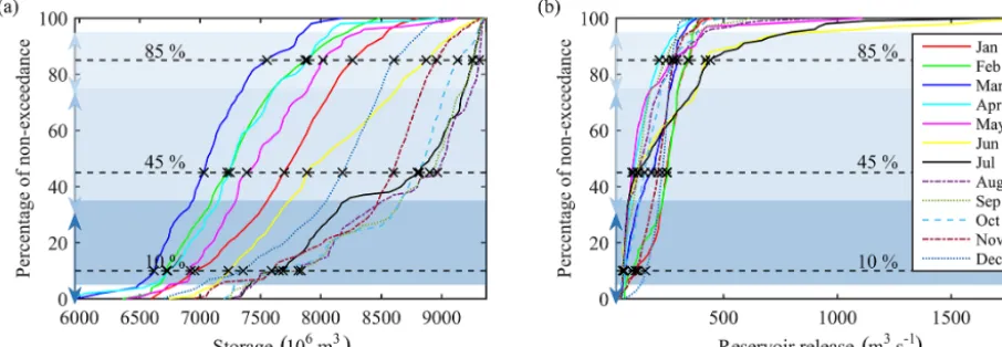
Qmi) that can vary for different times of the year. We rec-ommend varying these parameters on a monthly basis, while other time resolutions are also possible. To normalize the pa-rameters and their ranges across different types and sizes of reservoirs, for every reservoir, we use cumulative distribu-tion funcdistribu-tions (CDFs) of historical storage and release val-ues; see Fig. 2 for an example of CDFs of the Lake Diefen-baker reservoir (Gardiner Dam) in the Saskatchewan River basin, Canada. Our preliminary analysis indicated that target storage and release values corresponding to 10 %, 45 %, and 85 % non-exceedance probabilities generally perform rea-sonably well. We call these our generalized parameterization. However, optimal values of parameters for a given reser-voir can be identified, when data are available, through op-timization and parameter-identification techniques (Maier et al., 2019; Guillaume et al., 2019). For this purpose, we used a bi-objective optimization approach, as follows, that begins with the generalized parameter values as the starting point and optimizes the model fit to both storage and release data simultaneously:
F (x)=(f1(x), f2(x)) , (7)
where x is a vector of decision variables (parameter val-ues),is decision space,f1(x)is NSE (flow) measuring the
goodness of fit in reproducing observed release, andf2(x)is
NSE (storage) measuring the goodness of fit in reproducing observed storage dynamics.
For parameter identification on a monthly basis, a total of 72 decision variables were used in the optimization. We chose rather arbitrarily the storage and release target intervals that correspond to 5 %–35 %, 35 %–75 %, and 75 %–95 % non-exceedance probabilities as the ranges of variation for critical, normal, and maximum (flood) storage and release, respectively.
Figure 2.Cumulative distribution function (CDF).(a)Storage CDF of Gardiner Dam.(b)Reservoir-release CDF of Gardiner Dam. Double arrows onyaxis show parameterizations ranges for each generalized parameter.
3.4 Comparison of reservoir operation models
We compared the performance of our DZTR model against the performances of Hanasaki et al. (2006) and Wisser et al. (2010) using NSE and KGE performance metrics de-fined on both storage and release simulations. The compar-isons were made only for selected non-irrigation reservoirs because their irrigation reservoir formulation requires addi-tional data on water demands. For the method of Wisser et al. (2010), reservoir release was estimated under two condi-tions as shown in Eq. (8):
Qt=
κIt It≥Im,
λIt+(Im−It) It< Im, (8)
whereκ andλare empirical constants set to 0.16 and 0.6, respectively,Imis the mean annual inflow (m3s−1), andItis inflow to the reservoir (m3s−1) at timet.
In the method of Hanasaki et al. (2006), the release from non-irrigation reservoirs was estimated by multiplying the mean annual inflow by release-constraining coefficients (Eq. 9). The release-constraining coefficients for every given operational year were estimated by dividing the initial stor-age of that year by the maximum storstor-age (Eq. 10). The start of the operational year was considered to be the month when the mean monthly inflow shifts from being greater to being lower than the mean annual inflow:
rm,y=
(
krls,y·rm0,y (c≥0.5), c
0.5 2
·krls,y·rm0,y+
1− c
0.5 2
·im,y (0≤c <0.5), (9) krls,y=
Sfirst,y α·Smax
, (10)
where c is the ratio of maximum reservoir storage to the mean total annual inflow, krls,y is the release coefficient, rm0,y is the provisional monthly release (m3s−1) which is equal to mean annual inflow (m3s−1), and α is a dimen-sionless constant set to 0.85. Equation (12) differentiates
be-tween multi-year and single-year storage reservoirs based on a threshold value of 0.5 forc.
3.5 MESH modeling system
MESH is Environment and Climate Change Canada’s land-surface–hydrology modeling system (Pietroniro et al., 2007) and has been widely used in different parts of Canada (Davi-son et al., 2016; Haghnegahdar et al., 2017; Yassin et al., 2017; Sapriza-Azuri et al., 2018; Berry et al., 2017). MESH is a grid-based modeling system composed of three com-ponents: (1) the Canadian Land Surface Scheme (CLASS; Verseghy, 1991; Verseghy et al., 1993), (2) lateral movement of surface (overland) runoff and subsurface water (interflow) to the channel system within a grid cell, and (3) hydrological routing using WATROUTE from the WATFLOOD hydrolog-ical model (Kouwen et al., 1993).
et al. (2003), which was shown to be unsuitable for highly managed reservoirs. To improve the reservoir representation in MESH, this study aims to incorporate the DZTR model for controlled reservoirs into the MESH framework and evaluate its performance.
3.6 Case studies and data
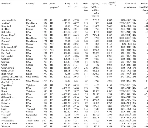
The dataset required to build and evaluate a reservoir op-eration model includes (1) reservoir physical characteristics such as the volume–level–area relationship and maximum capacity, which are static (in the absence of sedimentation or dam heightening), (2) time series of hydrologic variables such as inflow, release, and water level (or storage), and (3) environmental flows. In this study, we assembled such a dataset for 37 reservoirs located in several regions across the globe (Fig. 3) to test the model. These dams represent a wide range of storage sizes, from 0.132×10⁹to 162×109m3, spanning multiple orders of magnitudes. Most of these are lo-cated in the western US and western Canada, while some are located in Vietnam, central Asian countries, and Egypt. Ta-ble 1 provides a summary of reservoir locations, construction years, main purposes, data periods, and other dam character-istics. Measured inflow, release, and storage time series were collected from different sources. For reservoirs located in Canada, the data were acquired from Water Survey Canada, Alberta Environment and Parks, and the Saskatchewan Wa-ter Security Agency. Data for the High Aswan Dam were ac-quired from the Nile Basin Encyclopedia via the Nile Basin Initiative. The data for other reservoirs were provided by the authors of previous studies (Hanasaki et al., 2006; Coerver et al., 2018). Additional information about the degree of regu-lation, dam height, and catchment area were obtained from the GRanD database (Lehner et al., 2011). Reservoir opera-tion simulaopera-tions were performed on a daily and monthly ba-sis, with simulation periods varying from 8 to 62 years. The choice of simulation period and timescale was based on data availability (Table 1). The first year of the reservoir simula-tions was used for spin-up, while the first half of the remain-ing data periods was used for calibration and the second half for model validation.
[image:10.612.310.548.69.190.2]We also evaluated the integration of our reservoir model into the MESH model on seven reservoirs in two major basins in western Canada. Six of the test reservoirs (Gar-diner, St. Mary, Waterton, Oldman, Ghost, and Dickson dams) are located within the heavily regulated Saskatchewan River basin (SaskRB), and one reservoir (W. A. C. Ben-nett Dam) is located in the Mackenzie River basin (MRB). For both of the basins, the MESH model was set up on a grid resolution of 0.125◦, and the data required to build the MESH model were obtained from different sources. The to-pographic data are based on the Canadian Digital Elevation Data (CDED) at a scale of 1:250 000 and were obtained from the GeoBase website (http://www.geobase.ca/, last ac-cess: February 2018). The data on seven climate forcing
Figure 3.Locations of dams used to evaluate the reservoir routing model.
variables were obtained from a Global Environmental Mul-tiscale (GEM) numerical weather prediction (NWP) model (Côté et al., 1998) and the Canadian Precipitation Analy-sis (CaPA; Mahfouf et al., 2007). The land-cover data used are based on a 2005 land-cover map from the Canada Centre for Remote Sensing (CCRS). Soil texture data were obtained from Soil Landscapes of Canada (SLC) data of Agriculture and Agri-Food Canada. The MESH parameter values were taken from previous studies for calibration to streamflow at major subbasins of the SaskRB and MRB.
4 Results and discussion
4.1 Evaluation of the dynamically zoned target
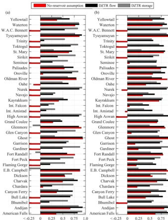
release (DZTR) model with generalized parameters Individual reservoir simulations were conducted using the DZTR model with generalized monthly storage and release parameter values set at non-exceedance probabilities recom-mended in Sect. 3.3 for representing the reservoir storage zones and their respective target releases. The evaluation of the DZTR model was based on the performance metrics and a comparison with the other reservoir operation approaches and a base case where the existence of a reservoir was ig-nored in a model, referred to as the “no-reservoir assump-tion”. Under the no-reservoir assumption, the release was considered equal to inflow, storage was considered constant, and, as such, the performance metrics were computed by di-rectly comparing inflow with observed release.
E. B. Campbell1 Canada 1963 HP −103.40 53.66 34 2200 0.153 2000–2011 (12) −1.69
Flaming Gorge1 USA 1964 WS −109.42 40.91 153 4336.3 2.460 1971–2017 (46) −6.37
Fort Peck1 USA 1957 FC −106.41 48.00 78 23 560 2.210 1970–19992(30) 6.33
Fort Randall USA 1953 FC −98.55 43.06 50 6683 0.240 1970–19992(30) −1.43
Gardiner Canada 1968 IR −106.86 51.27 69 9870 1.460 1980–2011 (32) −3.44
Garrison1 USA 1953 FC −101.43 47.50 64 30 220 1.436 1970–19992(30) −5.79
Ghost Canada 1929 HP −114.70 51.21 42 132 0.048 1990–2011 (22) 5.43
Glen Canyon1 USA 1966 HP −111.48 36.94 216 25 070 2.230 1980–1996 (17) −6.87
Grand Coulee USA 1942 IR −118.98 47.95 168 6395.6 0.124 1978–1990 (12) −3.37
High Aswan Egypt 1970 IR 32.88 23.96 111 162 000 2.843 1971–19972(26) −3.34
Amistad (Int. Amistad) USA–Mexico 1969 IR −101.05 29.45 87 6330 2.457 1977–2002 (25) −20.28 Falcon International
USA–Mexico 1954 FC −99.17 6.56 53 3920 1.045 1958–2001 (43) −14.48
(Int. Falcon)
Kayrakkum1 Tajikistan 1959 HP 69.82 40.28 32 4160 0.199 2001–20102(10) 1.19
Navajo USA 1963 IR −107.60 36.80 123 1278 1.744 1971–2011 (40) −21.07
Nurek Tajikistan 1980 IR 69.35 38.37 300 10 500 0.540 2001–20102(10) 0.28
Oahe Dam1 USA 1966 FC −100.40 44.45 75 29 110 1.244 1970–19992(30) −5.366
Oldman River Canada 1991 IR −113.90 49.56 76 490 0.446 1996–2011 (16) 3.98
Oroville1 USA 1968 FC −121.48 39.54 235 4366.5 0.804 1995–2004 (11) 4.20
Palisades USA 1957 IR −111.20 43.33 82 1480.2 0.242 1970–2000 (31) 0.48
Seminoe USA 1939 IR −106.91 42.16 90 1254.8 1.048 1951–20132(63) −4.10
Sirikit Thailand 1974 IR 100.55 17.76 114 9510 1.834 1981–1996 (16) −7.32
St. Mary Canada 1951 IR −113.12 49.36 62 394.7 0.492 2000–2011 (12) 0.16
Toktogul1 Kyrgyzstan 1978 HP 72.65 41.68 215 19 500 1.393 2001–20102(10) −6.34
Trinity USA 1962 IR −122.76 40.80 164 2633.5 1.470 1970–2000 (31) −4.18
Tyuyamuyun Turkmenistan NA IR 61.40 41.21 NA 6100 0.204 2001–20102(10) -2.43
W. A. C. Bennett Canada 1967 HP −122.20 56.02 183 74 300 1.200 2003–2011 (9) 5.41
Waterton Canada 1992 IR −113.67 49.32 55 172.7 0.258 2000–2011 (12) −10.34
Yellowtail USA 1967 IR −107.95 45.30 160 1760.6 0.489 1970–20002(31) −1.693
∗
Main purpose: WS – water supply, HP – hydropower, IR – irrigation, and FC – flood control.1Monthly data and simulation.2Multiple reservoir models that are compared on this reservoir. NA – not available.
are much lower than those of the DZTR model. Under the no-reservoir assumption, 48 % of the no-reservoirs resulted in a neg-ative NSE (base case). Almost all positive NSE (base case) results were observed in reservoirs with c <0.5, such as Dickson, E. B. Campbell, Kayrakkum, Oldman, and Tyuya-muyun (as explained in Sect. 3, cis the ratio of storage ca-pacity to annual inflow volume). However, for reservoirs with c >0.5, such as Bhumibol, Flaming Gorge, Fort Peck, High Aswan, and W. A. C. Bennett, the NSE (base case) is neg-ative, which indicates the significant influence of their reg-ulations on the hydrograph shape. Similarly, Fig. 4b shows the evaluation of the different reservoir models based on the KGE metric (Gupta et al., 2009). The values of KGE (flow) and KGE (storage) are greater than 0.25 and 0.5 for 100 %
and 86 % of the reservoirs, respectively. The KGE (base case) values of 21 % of reservoirs are less than zero, while those of 57 % and 49 % of the reservoirs are greater than 0.25 and 0.5, respectively. The NSE and KGE results show that the DZTR with the generalized parameter values is capable of simulat-ing flow and storage simulation well.
[image:11.612.50.544.85.515.2]ex-Figure 4.Performance evaluation result of the DZTR model reservoir operation algorithm:(a)NSE performance metrics and(b)KGE performance metrics.
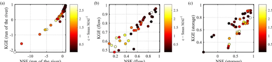
pected, the degradation of performance was pronounced for the no-reservoir assumption as the regulation level increased, while DZTR performance reduced by a much smaller extent (still positive values). Almost all low-regulation-level reser-voirs (c <0.5) showed positive performance metrics, which means that the reservoir regulation does not strongly mod-ify the flow regime, whereas the opposite case is true for highly regulated reservoirs (c >0.5) in which the reservoir regulation strongly changes the reservoir release. Coerver et al. (2018) also noted that low-regulation-level reservoirs are more dependent on the current time-step inflow knowledge because of their smaller influence on the flow regime. The method of Hanasaki et al. (2006) also recognizes the strong
dependence ofc <0.5 reservoirs on inflow to determine the release by configuring the release as a function of monthly mean inflow. Conversely, the relationship between the reg-ulation level and the storage simreg-ulation performance – in terms of both KGE (storage) and NSE (storage) – did not show a strong correlation (Fig. 5c).
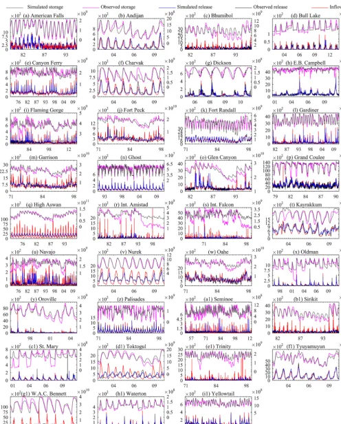
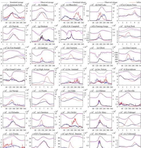
[image:12.612.129.467.64.505.2]monthly seasonality as well as the magnitude and timing of storage and releases for almost all reservoirs, especially for reservoirs with high regulation (multipurpose and multi-year reservoirs) such as American Falls, Bhumibol, High Aswan, Sirikit, Trinity, and W. A. C. Bennett dams. How-ever, the simulations also show some systematic over- and underestimations; for example, the simulations of Bhumibol, Fort Peck, High Aswan, Int. Falcon, Navajo, Bennett, and Int. Amistad reservoirs show continuous underestimation and overestimation of reservoir storage. Some reservoirs, such as Trinity, Palisades, Kayrakkum, Flaming Gorge, and Garri-son, show underestimation and overestimation of reservoir storage only for some seasons. A closer look at American Falls, Flaming Gorge, Fort Peck, Glen Canyon, and Navajo dams in Fig. 6 indicates that the DZTR model reliably cap-tured storage and release seasonality, inter-annual trends, and release pattern shifts during the consecutive wet years 1982– 1986 followed by consecutive dry years 1987–1993. Similar patterns can be observed for the Gardiner Dam, with good simulation results during both dry years (1984–1986, 1988– 1989, and 1999–2004) and wet years (1993, 2005, and 2010– 2011). Furthermore, as expected, Fig. 7 shows that lowly regulated reservoirs (c <0.5) have less of an impact on the flow regime, but with fairly significant storage seasonality (Oldman, E. B. Campbell, Palisades, and Andijan). In gen-eral, the DZTR model with the generalized parameterization of reservoir zones and releases showed an improved perfor-mance and can be applied to any hydrological model (CM or H-LSM) that involves reservoir simulation.
It is important to note that for the case of a cascade of reservoirs, the parameterization of the DZTR model implic-itly accounts, to some extent, for the upstream regulation ef-fects of the upstream cascade reservoirs. This is because the regulated inflow is used for parametrizing downstream reser-voirs, which reflects the regulation information of upstream reservoirs in the cascade. In reality, the operations of some cascade reservoirs are highly interlinked, particularly during the flood season. The decision regarding the release from one reservoir accounts for the (forecasted) state of other reser-voirs. Such dual- or multi-linked operation is, however, not accurately accounted for in the presented algorithm because
it assumes that each reservoir operates using its own stor-age state, inflow, and target storstor-age and releases. Such sys-tems require detailed modeling of operations that is not usu-ally attainable in large-scale hydrological models. Depend-ing on the purpose of the model, the modeler may decide to lump those reservoirs together to improve simulations down-stream, e.g., Ehsani et al. (2016).
4.2 Comparison with previously developed reservoir operation models
[image:13.612.72.528.66.171.2]Figure 7.Long-term average daily or monthly reservoir simulations with generalized parameterization; thexaxes show days (1–365) or months (1–12), the primaryyaxes show release (m3s−1), and the secondaryyaxis shows storage (m3).
The above comparisons were conducted for non-irrigation reservoirs because water demand data are needed to use the Hanasaki et al. (2006) method for irrigation reservoirs. In the case of the DZTR approach, the idea is that the DZTR model operates in such a way that it infers existing opera-tional rules that cater to those demands. Thus, the release from DZTR accounts implicitly for downstream demands as
per the intended purpose of the reservoir, whether it is for flood control, irrigation, hydropower, etc., or any combina-tion of these. The case study dams include reservoirs with different purposes, as shown in Table 1. The DZTR approach showed good performance for these reservoirs.
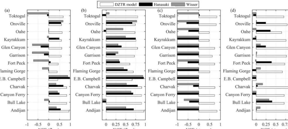
Figure 8.A comparison of our proposed reservoir operation model with generalized parameters with the models of Hanasaki et al. (2006) and Wisser et al. (2010):(a)NSE (flow),(b)KGE (flow),(c)NSE (storage), and(d)KGE (storage).
parameterization is optimized based on observed releases. The release from an irrigation dam will be available for abstraction at the predefined abstraction points downstream of the dam. The abstraction and distribution can be imple-mented as separate modules, as done within the MESH land-surface model (Yassin et al., 2019). In such an implementa-tion, MESH takes care of (1) calculation of actual irrigation demand for a configured irrigation area, (2) water abstraction from the defined abstraction point along the river below the dam, and (3) distribution across the irrigation fields. Regard-ing the return flow, the excess water flows from the irrigation areas are assumed to join the nearest stream within the model grid cell.
The DZTR model can in principle handle multipurpose reservoirs, e.g., a reservoir that is used simultaneously for hydropower generation, irrigation water supply, and flood control (e.g., High Aswan Dam in Egypt, which is one of the studied reservoirs); the DZTR provides the release based on the inflow and storage conditions that will be available for irrigation downstream. Hydropower does not consume water but returns it back to the river (except in rare cases where it returns to a different channel). Flood control is di-rectly accounted for in the scheme and becomes relevant when storage is within the flood storage zone. Further, the flexible formulation of DZTR allows for implicitly chang-ing the priorities in operation for selected time periods (e.g., months or seasons) by changing the target storage values during flood periods (e.g., the storage target before the on-set of snowmelt). During these flood months, lowering the target storage would increase the buffer for flood control. Conversely increasing the target storage during other months would be desirable to store water and release during
irriga-tion months. When the scheme is optimized using inflow, re-lease, and storage data, the parameterizations capture these priorities implicitly, as expressed in the data. When inflow data are lacking, the generalized parameterization will set the storage zones based on the suggested exceedance probabili-ties (that were deduced based on all reservoirs used in the study), and the priorities can be assumed as predefined. 4.3 Initial storage and inflow sensitivity test
The initial storage at the beginning of the simulation is an input that needs to be specified for the model. The initial values can be prescribed from the observations, if available. However, the simulation of a hydrological and land-surface model could start at any point in time when there is no obser-vation is available (e.g., some time in far past, a future sce-nario simulation, or a hypothetical scesce-nario). Additionally, in a long-term simulation, the initial storage may result from a previous model simulation, which may not be as close to observations as desired. The aim of the experiment is to ex-amine and show the extent to which the initial storage value affects the simulation performance.
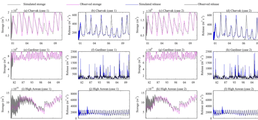
To test the effect of initial storage used in the reservoir simulation performance, two experiments were conducted on three reservoirs with different scales of regulations: (1) Char-vak (c=0.28), (2) Gardiner (c=1.46), and (3) High Aswan (c=2.84). In the first experiment, the initial storage was al-lowed to vary between 10 % of maximum storage (0.1·Smax)
and maximum storage (Smax). In the second experiment, the
diner Dam, this simulation reduced the NSE (flow) range to [0.49, 0.51] and the NSE (storage) range to [0.76, 0.87] in the first experiment and to 0.49 NSE (flow) and 0.87 NSE (stor-age) for the second experiments. On the other hand, the simulation on the High Aswan Dam showed a range of [−0.28, 0.85] for NSE (flow) and [0.38, 0.91] for NSE (stor-age) for the first experiment and [0.52, 0.85] for NSE (flow) and [0.42, 0.91] for NSE (storage) for the second experi-ment. Excluding a 1-year spin-up period from the metric cal-culation on the High Aswan Dam simulation narrowed the NSE (flow) range to [0.62, 0.85] and the NSE (storage) range to [0.58, 0.91] for both experiments. Overall, as expected, the experiments suggest that the effect of initial storage on reservoir simulation performance depends on the regulation scale. Starting from observed storage values and using a 1-year warm-up period allows stabilization of the initial stor-age effect for low and medium regulated reservoirs. How-ever, for highly regulated reservoirs, as in the case of High Aswan, longer spin-up periods are needed to stabilize the simulations. For example, a 5-year spin-up period was re-quired to fully stabilize the performance for the High Aswan Dam simulations.
The existence of inflow bias is inevitable in any hydro-logical modeling practice. To understand the behavior of the DZTR model under biased inflow conditions, we conducted a sensitivity experiment on the Charvak, Gardiner, and High Aswan reservoirs. To do so, the DZTR model performance was tested using five simulations in which the entire inflow time series was changed by−50 %,−25 %, 0 %,+25 %, and
+50 %. The sensitivity of simulations to bias in inflow was evaluated using the NSE (flow) and NSE (storage) perfor-mance metrics.
Figure 10 and Table 3 show the results of the inflow bias test and that the reservoir simulation performance signifi-cantly changes as a result of this bias. Reducing the inflow by 50 % considerably reduced the reservoir storage and release and led to negative values of NSE (flow) and NSE (storage) for all reservoirs. For such a large negative inflow bias, the reservoir operation tries to recover the storage to the target (observed) level by releasing as low as possible. Conversely, the positive inflow bias increased simulated storage and
re-the±25 % inflow bias significantly reduced the performance to negative values.
4.4 Parameter calibration and validation of the DZTR model
Figure 9.Reservoir initial storage effect on storage and release simulation:(a)Charvak storage case 1,(b)Charvak release case 1,(c)Charvak storage case 2,(d)Charvak release case 2,(e)Gardiner storage case 1,(f)Gardiner release case 1,(g)Gardiner storage case 2,(h)Gardiner release case 2,(i)High Aswan storage case 1,(j)High Aswan release case 1,(k)High Aswan storage case 2, and(l)High Aswan release case 2.
Table 2.Reservoir initial storage effect on storage and release simulation.
Case 2
S0= [min(obs) max(obs)], Case 1 obs=observed for all 1 Jan observations
S0=[0.1SmaxSmax] from the historical reservoir storage data
NSE NSE NSE NSE
(storage) (flow) (storage) (flow)
Charvak No spin-up [0.61 0.74] [0.79 0.83] [0.61 0.74] [0.79 0.83] 1 year spin-up [0.74 0.74] [0.82 0.82] [0.74 0.74] [0.82 0.82]
Gardiner No spin-up [−0.43 0.88] [0.35 0.51] [0.87 0.88] [0.44 0.49] 1 year spin-up [0.76 0.87] [0.49 0.51] [0.87 0.87] [0.49 0.49]
High Aswan No spin-up [0.38 0.91] [−0.28 0.85] [0.42 0.91] [0.52 0.85] 1 year spin-up [0.58 0.91] [0.62 0.85] [0.58 0.91] [0.62 0.85]
56 % of the reservoirs, with a median improvement of 0.035 and 0.092, respectively. The NSE (flow) improvement in the validation period ranged from 0.001 to 0.335, and NSE (stor-age) improvement ranged from 0.004 to 1.02. During vali-dation, the remaining reservoirs (44 % of them) resulted in NSE (flow) and NSE (storage) reductions, with a median reduction of 0.032 and 0.089, respectively. The reductions of NSE (flow) ranged from 0.001 to 0.073, and those of NSE (storage) ranged from 0.001 to 0.257.
Overall, considerable improvement was achieved for both calibration and validation periods for several reservoirs, such as the Dickson, Gardiner, Ghost, Int. Amistad, Int. Falcon, Kayrakkum, Sirikit, Yellowtail, and Glenmore. However, as
[image:18.612.90.508.378.542.2]Figure 10.Inflow bias sensitivity test on storage and release simulation:(a)Charvak storage,(b)Gardiner storage,(c)High Aswan storage, (d)Charvak release,(e)Gardiner release, and(f)High Aswan release.
Table 3.Inflow bias sensitivity test on storage and release simulation.
−50 % −25 % 0 % 25 % 50 %
Charvak NSE (storage) −1.95 0.25 0.74 0.52 −0.21 NSE (flow) −0.06 0.54 0.82 0.57 −0.07
Gardiner NSE (storage) −2.00 0.74 0.88 0.79 0.66 NSE (flow) −0.21 0.47 0.49 −0.43 −2.02
High Aswan NSE (storage) −9.37 −5.96 0.90 −0.60 −1.45 NSE (flow) −3.90 −0.34 0.80 −2.29 −8.70
degradation during the validation period. In general, a small change in inflow, storage, or release for the validation pe-riod can change the shape of the trade-off. However, the cali-brated parameters in most cases were still capable of produc-ing good performance durproduc-ing validation that was close to, or better than, that of the generalized parameterization for the same period.
To further test the role of the calibration period, we cal-ibrated all reservoirs using the whole observational record. The result of this test is shown in Fig. 12, which demon-strates the strong role of the calibration period. All reservoirs showed trade-off between storage and release fitting. The so-lution resulted in a consistent Pareto pattern similar to the split-sample calibration results. The median NSE (flow) and NSE (storage) improvement when using the whole observa-tional record for calibration is approximately 0.1 and 0.12 respectively, while the maximum improvement reached 0.45 and 0.55 for some reservoirs. High improvements in stor-age and flow simulations in the case of whole-period cali-bration are mostly observed in reservoirs that have
[image:19.612.151.445.356.457.2]Figure 11.Reservoir-release-parameter multi-objective calibration result.xaxes show NSE (flow) multiplied by−1, and theyaxes show NSE (storage) multiplied by−1.
The DZTR scheme introduces more parameters to the host land-surface model. However, its parameters are external to those of land-surface model and are determined a priori us-ing storage and release data. The decision of the timescale to use for specifying the parameters is left to the modeler. The
Figure 12.Reservoir-release-parameter multi-objective calibration using all available data for each reservoirs;xaxes show NSE (flow) multiplied by−1, and theyaxes show NSE (storage) multiplied by−1.
information, or zoning values specified in other studies, such as that of Zhao et al. (2016).
4.5 DZTR model test within the MESH model
Figure 14.Long-term average daily or monthly reservoir simulations with generalized parameterization; thexaxes show days (1–365) or months (1–12), the primaryyaxes show release (m3s−1), and the secondaryyaxes show storage (m3).
St. Mary, Waterton, Oldman, Ghost, and Dickson dams) and one reservoir (W. A. C. Bennett Dam) in the Mackenzie River basin, both in Western Canada. The reservoir simulation was run using MESH-modeled inflows at a half-hourly time step, the usual MESH time step, and the performance metrics were calculated at a daily time step. The MESH-modeled inflows are considered to represent the base-case scenario, and the
inflow can be assumed to be regulated or natural, depending on whether there are dams upstream or not.
in NSE. The importance of integration of the DZTR model was predominant for the Gardiner and W. A. C. Bennett dams, which are highly regulated reservoirs (c >0.5) when compared to the other reservoirs tested in MESH.
This general improvement of flow simulation when com-paring a reservoir model to the no-reservoir assumption is, of course, not surprising. What is important to note, how-ever, is that the improvement in NSE can be substantial with-out calibration of the DZTR parameters. This is important for many LSM applications where calibration is generally not performed. Hanasaki et al. (2006) illustrated that their method is superior to the natural lake (or unregulated reser-voir) method applied in many CMs and H-LSMs, and this paper shows that the DZTR model improves upon the results of Hanasaki et al. (2006). Therefore, it is natural to assume that the DZTR model would also be an improvement in un-calibrated H-LSM applications.
However, calibration is very common in CM or H-LSM applications in which the DZTR model would likely be em-ployed. A full comparison of calibrated results between a no-reservoir case, natural lake (or unregulated no-reservoir), and the DZTR model (and the other reservoir models) is be-yond the scope of this paper. Again, given the improvements shown with the uncalibrated DZTR model when compared with other uncalibrated models, and the general improve-ments shown here when calibrating the DZTR model, it is assumed that calibrating the DZTR model within a CM or H-LSM would improve upon calibrating an unregulated reser-voir model or the other reserreser-voir models compared in this paper.
The storage simulation showed a low NSE (storage) value for the St. Mary and Waterton dams and a negative NSE (stor-age) for Oldman and Ghost dams. However, the simulation showed a reasonable representation of storage variability but with considerable underestimation. This underestimation in storage in Fig. 15 is attributable to the fact that the modeled inflow is underestimated. It is expected that calibration of the land-surface parameters in conjunction with the DZTR pa-rameters in MESH would improve the modeled inflows and resulting modeled reservoir storage.
It is worth mentioning again that H-LSMs, such as MESH, can also be used for the original purpose of LSMs, which is to represent fluxes from the land-surface to the atmosphere. If the approach improves modeled flows where reservoirs op-erate, it could result in a better parameterization of the LSM, which should in turn improve land-surface fluxes and feed-backs to the atmosphere.
4.6 Uncertainties in reservoir operations and DZTR parameterization
Reservoir operation involves considerable uncertainties that several factors are attributed to. One major source of uncer-tainty in reservoir operations is future inflows (long-term and short-term inflow forecast). The forecast contains errors are
rooted in the forecast method, the driving climate forecast, snowpack measurements, timing of snowmelt, and the sta-tistical (stationarity) assumptions to generate inflows based on historical inflows. The inflow forecast uncertainty is more significant during flood seasons because it involves subjec-tive decisions of operators to avoid the risk of dam overtop-ping and downstream flooding. Other sources of uncertainty in reservoir operations include changes in demand over time because of increases in demand for irrigation, power, wa-ter supply, etc. The purpose of the reservoir can also change from its initial intended purpose (e.g., adding a hydropower station to an irrigation dam). These changes are only implic-itly captured by the DZTR scheme, as implied in the storage and release time series used for parameterizing it for a spe-cific reservoir.
Given the above uncertainties, even the actual reservoir operation may deviate from the designed reservoir tion rule curve. Some of the decisions of reservoir opera-tors are spontaneous, ad hoc, and depend on experiences that are not usually documented. Thus, there are difficulties in accurately representing the historical operation or establish-ing accurate relationships between reservoir storage, inflow, and release. These relationships typically contain consider-able noise, e.g., different release values for the same storage level during the same season. As a result, these uncertainties influence considerably the parameterization of the model de-rived to represent the reservoir operation based on historical observations of each reservoir. This is particularly true for the algorithm presented because of two main factors. Firstly, the presented reservoir algorithm assumes that the relationship between reservoir storage and releases follows piecewise-linear functions. There is a chance that other functional forms represent such relationships better for some reservoirs. Sec-ondly, in the case of the generalized parameterization, the bending points in the piecewise linear functions (zone classi-fication points) are estimated based on fixed probabilities of exceedance extracted from historical data for all reservoirs. A different dataset (of reservoirs and/or time periods) could result in different quantiles. The assumption of having sim-ilar bending points of the piecewise-linear functions for all reservoirs cannot provide optimal zones for each reservoir. However, we showed that the generalized parameterization performs better compared to other widely used algorithms.
Figure 15.Reservoir simulation results within MESH model run for selected reservoirs;xaxis shows time (d), the primaryyaxes show release (m3s−1), and the secondaryyaxes show storage (m3).
of the limitation of the reservoir algorithm (piecewise linear functions, fixed number of zones, etc.) and observation er-rors. To examine the level of uncertainty of the trade-off, it is important to look at the shape and range of the trade-off on each objective function axis.
As shown in Figs. 11 and 12, apart from a few reservoirs, the range of Pareto solutions for each objective function is generally narrow, with good NSE values (Figs. 11 and 12). In such cases, the associated uncertainties are few, and the trade-off between improving simulated releases and improv-ing simulated storage is minimal. Conversely, in some cases, an extended spread of the trade-off along one of the axes (objective function) was observed, indicating a higher uncer-tainty of the algorithm for the process that the axis repre-sents, i.e., reservoir storage or release. This requires further investigation of the datasets and parameterization for those reservoirs and their history of operations. Shifts in opera-tional management of reservoirs do occur, and these may ob-scure the parameterization. These may be detected by care-ful examination of the available records as well as metadata records of the reservoir history if accessible. The level of noise when determining the parameters could be an indicator of changes in operation.
4.7 Implementation strategies to overcome data limitation
The data requirement is the main limitation of the DZTR model for application at continental and global scales. One approach to overcome data limitations is to integrate our pro-posed method in land-surface and catchment models along with other reservoir operation methods (e.g., Hanasaki et al., 2006). Then, within the land-surface and catchment models, identifier flags can be used to indicate which method applies to which reservoirs. The DZTR approach can only be acti-vated for reservoirs with data support, while the remaining reservoirs can use other approaches as dictated by data avail-ability. We follow such an implementation within the MESH model.
have a better understanding of the system to acquire the nec-essary reservoir data. In a land-surface hydrologic model, important reservoirs are those causing large changes to the downstream flows, and those tend to be the larger ones with generally better data availability.
Data on reservoir storage, inflow, and release exist for most reservoirs, but sometimes they are not made publicly available. Storage data can be obtained from water-level data, which are generally available for major reservoirs and can be converted to storage. Release data can be deduced from the nearest downstream station. In addition, new initiatives are needed to gather and archive such reservoir datasets and move beyond the information on reservoir characteristics that is currently available in databases (e.g., GRanD database – Lehner et al., 2011). One of our recommendations is that the target release and storage data be archived for public use at least for highly regulated and multi-year type dams (c >0.5). The possibility of estimating storage and release data from different satellite data products is promising; such new data sources will potentially improve the use of methods like the presented reservoir operation (optimized or generalized). More recently, Busker et al. (2019) showed an estimation of volume for 130 reservoirs using surface water dataset and satellite altimetry; this is an encouraging approach for reduc-ing data limitation.
5 Summary and conclusions
Human interventions in hydrologic systems through dams and reservoirs significantly change the flow regime of many rivers. In this paper, we presented an improved reservoir operation model, called the dynamically zoned target re-lease (DZTR) model, that can be integrated into any large-scale hydrological model; here we integrated it into the MESH land-surface–hydrology model. The DZTR model is based on parametric piecewise-linear functions that approxi-mate reservoir-release rules used by reservoir operators. We proposed two strategies to identify the parameters of this model: one based on the distributions of historical storage and release to generate the so-called generalized parameters and the other one based on direct calibration to observed stor-age and release time series via multi-objective optimization. We first tested the DZTR model individually across a num-ber of reservoirs around the globe and then tested its perfor-mance when plugged into the MESH model for a subset of those reservoirs. Our conclusions can be summarized as fol-lows:
– The DZTR reservoir operation model performed well in reproducing observed storage and release time se-ries in (almost) all reservoirs tested and outperformed the existing reservoir models proposed by Hanasaki et al. (2006) and Wisser et al. (2010). The model was ca-pable of capturing inter- and intra-annual variability in both reservoir storage and release.
– As expected, calibration significantly improved the formance of the DZTR model compared with the per-formance of the generalized parameters. However, a sig-nificant trade-off exists between fitting reservoir storage versus release, signifying the importance of accounting for both storage and release in a multi-objective fashion. – The integration of the DZTR reservoir model into the MESH land-surface–hydrology modeling system was straightforward and improved the overall model perfor-mance compared with the traditional methods of ac-counting for reservoirs in H-LSMs. This integration can be viewed as a successful example for improving the representation of reservoir operation in CMs, LSMs, and GWSMs.
Future research work may include (1) examining the appli-cability of the DZTR model for regions with severely limited data by examining the utility of other data sources such as those derived from satellite-based observations (Savtchenko et al., 2004; Garambois and Monnier, 2015; Gao et al., 2012) and using the area–volume relationship approximated by reg-ular geometric shapes (e.g., Yigzaw et al., 2018) and (2) ex-amining direct one-way and/or two-way coupling of WMMs with CMs and LSMs for developing a seamless coupled framework for the simulation of naturally engineered water-shed systems.
Data availability. Data used can be found in Yassin et al. (2018).
Author contributions. FY developed the methodology together with SR and HW. FY and GSA wrote all the computer codes cou-pled with the MESH model. FY designed the experiments and per-formed them all. FY was responsible for the verification of the re-sults. FY prepared the paper, and other co-authors contributed to editing of the paper at all stages.
Competing interests. The authors declare that they have no conflict of interest.
Special issue statement. This article is part of the special issue “Understanding and predicting Earth system and hydrological change in cold regions”. It is not associated with a conference.