www.hydrol-earth-syst-sci.net/14/545/2010/ © Author(s) 2010. This work is distributed under the Creative Commons Attribution 3.0 License.
Earth System
Sciences
Coupled hydrogeophysical parameter estimation using a sequential
Bayesian approach
J. Rings, J. A. Huisman, and H. Vereecken
ICG 4 – Agrosphere, Forschungszentrum J¨ulich, Germany
Received: 25 September 2009 – Published in Hydrol. Earth Syst. Sci. Discuss.: 15 October 2009 Revised: 26 February 2010 – Accepted: 17 March 2010 – Published: 18 March 2010
Abstract. Coupled hydrogeophysical methods infer hydro-logical and petrophysical parameters directly from geophys-ical measurements. Widespread methods do not explicitly recognize uncertainty in parameter estimates. Therefore, we apply a sequential Bayesian framework that provides updates of state, parameters and their uncertainty whenever measure-ments become available. We have coupled a hydrological and an electrical resistivity tomography (ERT) forward code in a particle filtering framework. First, we analyze a syn-thetic data set of lysimeter infiltration monitored with ERT. In a second step, we apply the approach to field data mea-sured during an infiltration event on a full-scale dike model. For the synthetic data, the water content distribution and the hydraulic conductivity are accurately estimated after a few time steps. For the field data, hydraulic parameters are suc-cessfully estimated from water content measurements made with spatial time domain reflectometry and ERT, and the de-velopment of their posterior distributions is shown.
1 Introduction
In recent years, the worth of geophysical methods in hy-drological applications has increasingly become apparent (e.g. Hubbard et al., 1999; Rubin and Hubbard, 2005; Linde et al., 2006; Vereecken et al., 2006). Typically, hydro-logical investigations rely on methods that disturb the soil, like soil coring, tensiometry or Time Domain Reflectometry (TDR). In contrast to that, non-invasive geophysical mea-surements provide the possibility to eavesdrop on subsur-face flow and transport processes without disturbing them.
Correspondence to: J. Rings ([email protected])
This way, spatio-temporal patterns of hydrological states can be retrieved. In hydrogeophysical applications, hydrological states and parameters are estimated through observations of geophysical states (e.g. electrical resistivity). The possibly unknown parameters encompass both hydrological parame-ters determining flow and transport and petrophysical param-eters that relate geophysical and hydrological state variables. Geophysical surveys conducted to estimate subsurface states or parameters have been approached in a three-step manner (see e.g. Binley et al., 2002; Kemna et al., 2002; Chen et al., 2004; Cassiani and Binley, 2005; Koestel et al., 2008; M¨uller et al., 2010). First, a geophysical survey re-trieves the geophysical state variables of the subsurface (e.g. the electrical resistivity distribution). Next, a petrophysical relationship is applied to transfer these into hydrological state variables (e.g. water content or tracer concentration). Finally, these state variables are used to drive a hydrological model or they are used in a parameter estimation process.
Integrated or coupled inversion approaches aim at infer-ring hydrological properties directly from the geophysical measurements. The parameters of the hydrological model and of the local-scale petrophysical relationship between geophysical and hydrological states are perturbed to mini-mize the difference between modelled and measured data. Several authors have investigated coupled hydrogeophysical inversion for hydrological modelling (Kowalsky et al., 2004; Lambot et al., 2006; Jadoon et al., 2008; Rucker, 2009; Hin-nell et al., 2010). These contributions used synthetic data to evaluate the usefulness and applicability of coupled in-version for simplified hydrological systems. Additionally, newer studies are increasingly applying these methods to actual field data, where the structural inadequacies of the models, measurement errors and the assumptions inherent to the petrophysical relationship complicate the inversion problem (Kowalsky et al., 2005; Deiana et al., 2008; Looms et al., 2008). In a recent contribution, Huisman et al. (2010) have formulated the coupled inversion problem in a Bayesian framework to explicitly recognize uncertainty. They argued that the posterior uncertainty of the model parameters and predictions is useful to explore the value of different mea-surement types.
The coupled hydrogeophysical approach is especially suited for problems where hydrological states are observed by geophysical measurements on several occasions (i.e. time-lapse geophysical surveys). When time-time-lapse geophysical measurements are used to monitor hydrological processes and to parameterize hydrological models, an inevitable ques-tion is whether addiques-tional measurements still provide addi-tional information to improve the hydrological model pa-rameterization. Although Huisman et al. (2010) showed that a Bayesian framework is useful to address this question, their framework only allows an answer a posteriori. For long-term monitoring, it is more attractive to provide regular updates of hydrological states, parameters and their uncertainty, using the information that is available so far.
Typically, filtering techniques, such as the popular Kalman filter (Kalman, 1960; Chen, 2003) are applied to update states whenever new measurements become available (e.g. Sepp¨anen et al., 2001). The classical Kalman filter relies on linear behaviour in time, but additional filters have been de-veloped that alleviate this problem, e.g. the extended Kalman filter (see e.g. Kaipio and Somersalo, 2004) or the ensemble Kalman filter (Evensen, 1994). Lehikoinen et al. (2009) have applied the extended Kalman filter to the problem of dynam-ical ERT inversion with explicit recognition of state uncer-tainty. However, all Kalman-type filters rely on Gaussian error distributions in the prior distribution.
A related family of filters are the particle filters. These filters are based on a sequential Bayesian framework (Gor-don, 1993; Doucet and de Freitas, 2001; Arulampalam et al., 2002; Storvik, 2002; Chen, 2003; Cappe et al., 2007). They have been designed to cope with arbitrary prior distributions. The posterior probability distributions are approximated by
sampling at discrete supporting points carried by weighted particles. This method is highly attractive for continuous state monitoring and also has potential for parameter esti-mation. A major advantage in a hydrogeophysical monitor-ing application is that the filter provides updated posterior distributions of states and parameters immediately after each measurement. Particle filters have recently been introduced into hydrology (see e.g. Weerts and El Serafy, 2006; Zhou et al., 2006; Hsu et al., 2009). Although filtering techniques are traditionally used to update state variables, they have also been applied in conjunction with hydrological models for parameter estimation (Kivman, 2003; Moradkhani et al., 2005; Vrugt et al., 2005; Hendricks Franssen and Kinzel-bach, 2008; Salamon and Feyen, 2009).
In this study, we apply particle filtering to the problem of estimating hydraulic and petrophysical parameters from ERT measurements made during infiltration in the unsatu-rated zone. The rest of this study is organized as follows. First, we introduce the concept and implementation of the particle filter. Next, we apply the particle filter to estimate the water content distribution and the saturated hydraulic conductivity from a simple synthetic data set consisting of ERT measurements made during infiltration into a lysime-ter. Finally, we apply the particle filter to estimate hydraulic and petrophysical parameters from ERT measurements made during infiltration into a full-scale dike model. As a refer-ence, we also determine these parameters from detailled spa-tial time domain reflectometry (TDR) measurements.
2 Methods 2.1 State models
We want to describe the state x of a system, in our case e.g. a vector containing water content or pressure head for each element of a discretized representation of the subsur-face. We can apply Bayesian analysis at each time step T=1,...,t,t+1,...At timet, this analysis can estimate past statesx1,...,xt−1(smoothing), the current statext(filtering) or the future statext+1(forecasting).xcan be seen as a ran-dom variable in a stochastic model that translates the state in time:
xt+1=f (xt,ξ,ut)+αt+1 (1)
where the operatorf is the time propagation function that translates the state in time fromttot+1 driven by some ex-ternal forcingut and modified by some static parametersξ. αt+1is Gaussian noise term that adds a stochastic diffusion process to the translation.
From a state xt+1, we can deduce an observation yt+1
yt+1=g(xt+1,ξ)+βt+1 (2) wheregis an operator to determine the system response from state and parameters, andβt+1again is a Gaussian term de-scribing the measurement noise. The noise term αt+1 and βt+1are assumed to be independent random vectors. 2.2 Parameter estimation
The state-space has been formulated in the previous section, where we assumed the parametersξ to be static. However, in this study we want to focus on parameter estimation rather than only filtering or forecasting of states. Therefore, we use a series of parametersξt, that shall converge to estimates of the true static parametersξ for t→ ∞. We assume these
ξt to be pseudo-static, meaning that they are not modified by external forcing, but only perturbed by a small Gaussian noise process as
ξt+1=ξt+ζt+1 (3)
whereζt+1is an independent Gaussian random vector im-plemented as a static noise term as suggested by Liu and West (2000). For simplification, we abbreviate the notation asz=(x,ξ), wherezis also known as the augmented state variable.
2.3 Sequential Bayesian filtering
Given the prior distribution of state and parameters p(z0:t+1), we can obtain the posterior distribution from fil-tering through the Bayesian theorem
p(z0:t+1|y1:t+1)=p(y
1:t+1|z0:t) p(z0:t+1)
p(y1:t+1) (4)
wherep(y1:t+1|z0:t)is a likelihood function for observations given the previous states andp(y1:t+1)is the normalization factor.
We approximate this pdf by a discrete set ofn=1...N par-ticleszi by assigning a weightwˆi to each particlei. Then,
we can write: p(z0:t+1|y1:t+1)=
N
X
i=1 ˆ
wit+1δ(z0:t+1−z0i:t+1) (5) whereδ()are Dirac delta functions. Initially, all particles are assigned the same weightwˆ0i =1/N.
Direct sampling from this posterior is generally very de-manding or impossible, so we rather sample from a known distributionq(z0:t+1|y1:t+1) called a proposal distribution.
This way, we can define new weightswias
wki+1=p(z
0:t+1|y1:t+1)
q(z0:t+1|y1:t+1). (6)
The choice of a proposal distribution is a critical decision (Arulampalam et al., 2002; Moradkhani et al., 2005), and is conveniently taken to be equal to the prior distribution q z0i:t+1|z0i:t,y1:t+1=p z0:t+1|z0i:t. (7)
The last step towards a sequential formulation is the assump-tion that the proposal distribuassump-tion is chosen so that it factor-izes in a recursive way:
q(z0:t+1)=q(z0:t|y0:t)q(zt+1|z0:t,yt+1) (8) By combining Eqs. (7) and (8), we arrive at the simple form for weight updating
wti+1=witp yt+1|zti+1
. (9)
Due to the Markovian formulation of the time propagation model in Eqs. (1) and (3) and the observation model in Eq. (2), this is a valid formulation and can be used to im-plement a particle filter.
2.4 Particle filter implementation
We implement a Sampling Importance Resampling (SIR) fil-ter, which basically follows a three-step approach. The first step is the time propagation of state and parameters which samples the evolution densityp(zt+1|zt)and follows from the models in Eqs. (1) and (3).
The second step is filtering, which assigns weights to the particles based on the probability for an observation. The observation is deduced from Eq. (2), then the weight is up-dated according to Eq. (9). In the case that measurements from j =1,...,J different sources are available, we have vectorsYj of measurement data (e.g. measured transfer
re-sistances or water content) and the modeled observationsyj, we evaluate the weight wi,j as the inverse of the distance
|Yti,j−yti,j|. If we assume to know the normalized, rela-tive measurement error rj of each method, we can obtain
wi=Pjrjwi,j. However, the filters implemented in this
study have been restricted to one measurement method. After assigning and normalizing the weightswi,
resam-pling is used to prevent a concentration of weights in only one or a few particles. To find out whether this is necessary, an effective particle numberNeis determined as
Ne=
X
i
w2i −1
. (10)
IfNeis larger than a threshold valueτ (e.g.τ=0.5), the
par-ticle set remains unchanged. Otherwise, this is an indication that the particle set has become impoverished, as few par-ticles contribute with considerable weight. To remedy this, a new set of particles is determined using a resampling al-gorithm. Douc et al. (2005) evaluated different resampling techniques, and found that the residual resampling technique (Liu and Chen, 1998) performed well. This resampling tech-nique allocates
n0i= bN wic (11)
copies of particlei in the new set and samples the remain-ingL=N−P
in
0
i particles from the multinomial distribution
Mult(L; ˜w1,...,w˜N)with
˜
wi=
N wi−n0i
The weightwi for all new particles is again set towi=1/N.
ForT→∞andN→∞, the posterior is found so that the weighted averageξ represents an appropriate parameter esti-mate:
ξ=X
i
wiξi (13)
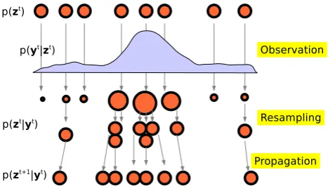
Figure 1 illustrates the particle filter method. We start with a particle cloud that has been propagated to timet. In the observation step, the particles are weighted according to how well they fit with the data. Then, they are redistributed ac-cording to their weights. A particle that has gained weight during observation may split up into two or more new par-ticles, and particles that had small weight after observation may be removed from the cloud. Finally, the propagation car-ries the particle states to timet+1, which in our case would mean a forward model run from timet tot+1. These steps are repeated as long as new measurements become available. 2.4.1 Time propagation
For each particlei, the functionf in Eq. (1) is evaluated by a hydrological forward model run from timet tot+1. The statexit enters as the initial water content or pressure head at timet.
The hydrological models used in this study are HYDRUS (e.g. Simunek et al., 2008) for 2-D modelling domains and PARSWMS (Hardelauf et al., 2007) for 3-D modelling do-mains. They solve the Richards equation for unsaturated water flow using a linear Galerkin approach in a finite el-ement scheme. We assume that the parametric model by van Genuchten (1980) can describe soil water retention and hydraulic conductivity as:
Seff=
θ−θr
θS−θr
=(1+ |αh|n)−m (14)
k(h)=kS
p Seff
h
1− 1−Seff1/mmi2
(15) where h is matrix potential (m), θ is the volumetric wa-ter content (m3/m3), θ
r is the residual water content for
h→−∞,θS is the saturated volumetric water content, αis
the inverse of the air-entry value (m−1), n is an empirical
shape factor (–), mis a factor that can be connected to n viam=1−1/nandkS is the hydraulic conductivity atθ=θS
(m/s).
2.4.2 Observations
[image:4.595.312.546.62.198.2]To evaluate particle weights, the modelled observationyhas to be determined. In this study, we concentrate on ERT as the geophysical observation method. To model the transfer resistances that are measured during an ERT survey, we have to determine the distribution of bulk resistivityρb from the
Fig. 1. Illustration of the filtering steps of observation and
prop-agation and the resampling scheme. Adapted from Chen (2003).
soil water content distribution. Therefore, the petrophysical relationship by Archie (1942) is used:
ρb=ρw8−mA
θ
8 −nA
(16) whereρw is the pore water resistivity (m), which is the
inverse of the pore water conductivityσw,8is the porosity
of the soil (m3/m3),mAis the cementation exponent (–) and
nA is the saturation exponent (–). Ulrich and Slater (2004)
determined saturation exponents ranging from 1.0 to 2.7 for unconsolidated sands.
We use an ERT forward code by Ruecker et al. (2006) for 3-D modelling domains and the CRMOD code (Kemna et al., 2000) for 2-D modelling domains. Both ERT for-ward models were coupled to hydrological models following the approach and considerations presented in Huisman et al. (2010).
3 Numerical experiment
As a proof of concept, we use a synthetic data set of simulated lysimeter infiltration monitored by cross-borehole ERT. The model domain was set up as a cube of 1 m edge length filled with a homogeneous material (withθr=0.001,
θS=0.27,kS=0.0015 m/s,α=4 andn=4.56). On each
Water was infiltrated from all surface nodes into an ini-tially dry medium (pressure headh=−1 m). Aftert=500 s, the wetting front reached the bottom of the volume. Arti-ficial measurements were created every 100 s with the ERT forward model. For this simulation, a coarser internal ERT forward grid was used as recommended by Kaipio and Som-ersalo (2004). The measurements were perturbed with 3% Gaussian noise.
3.1 Implementation of the particle filter
For this 3-D simulation, the hydrological model PARSWMS (Hardelauf et al., 2007) was coupled to the ERT forward code by Ruecker et al. (2006). The state vector was initialized uniformly for each particle with 1331 pressure head values (one for each grid node) and a variablekS. The initial state
and parameter distribution were sampled from uniform dis-tributions for N=1000 particles. Distribution bounds and true values can be found in Table 1. The particle filter has been realized in a wrapper software code “Particle Filter-ing Inversion-Friendly Framework” (PFIFF) implemented in Python that connects the coupled models with the propaga-tion, observation and resampling schemes.
For time propagation from t to t+1, the hydrological model was run conditional to the particle’s parameter kS.
Then, α=ζ=2% Gaussian noise were added to the aug-mented state to simulate a stochastic diffusion process.
We assumed that the petrophysical relationship was known, and used it to transfer soil water content to bulk resis-tivity for each cell. The resisresis-tivity distribution thus obtained was used in the filtering step to simulate an ERT measure-ment at timet+1. Then, particle weights were assigned and normalized. Finally, the particles were resampled (each time step, so that the resampling threshold wasτ=1) and their weights reset to 1/N.
3.2 Results
Figure 2 shows the distribution of particle weights immedi-ately before the first resampling (t=100 s) and at the end of the simulation (t=500 s). The figure implicitly contains the variability in the state estimate, as can be seen from differ-ent weights of particles with similar conductivity. The initial distribution of the states was only1h=4 cm wide, so it is evident that errors in the state have a large influence on the weight. While most particles have a low weight, some parti-cles near the true value ofkS=0.0015 m/s have a markedly
higher weight. At the final time step,t=500 s, the filtering and resampling have caused most particles to converge to the correct value. The weighted average ofkS is 0.00165 m/s,
[image:5.595.310.544.88.145.2]which is a slight overestimation. The state variable is shown for a 1-D vertical profile taken in the middle of the model do-main for two time steps (Fig. 3). The initial distribution was sampled from an interval that underestimated the pressure head (see Table 1) for all particles. While at timet=300 s, the
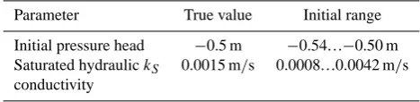
Table 1. Initial state and parameter value and range.
Parameter True value Initial range
Initial pressure head −0.5 m −0.54...−0.50 m Saturated hydraulickS 0.0015 m/s 0.0008...0.0042 m/s
conductivity
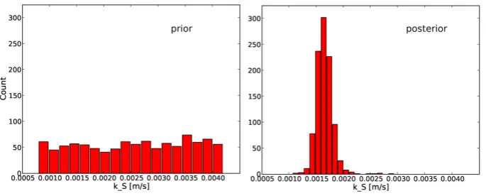
particle states show an even greater variability than in the ini-tial distribution, the true state (blue line) is no longer on the boundary of the distribution, but the particles gather around it. This is true not only for the model parts near the surface, where changes due to the infiltrating water front have influ-enced the particle states, but also near the bottom, where the stochastic diffusion process that is added to the time prop-agation step combined with the resampling have influenced the particle states to move into the right direction. In the final time step, att=500 s, the mean state value of all particles suc-cessfully retrieved the true state. Only in the lowest parts of the model (where ERT sensitivity is very low), the variabil-ity in pressure head is much higher. Finally, the results of the parameter estimation are shown as a comparison of the ini-tial prior and posterior pdf ofkS in the histograms in Fig. 4.
The prior distribution was randomly sampled from a uniform distribution, but the parameter estimation successfully trans-formed the pdf into a posterior distribution approximating a Gaussian distribution with a mean near the true value.
4 Full-scale dike model
4.1 Site description and measurements
Measurements have been taken on a full-scale dike model (see Fig. 5) located at the Federal Waterways Research In-stitute in Karlsruhe, Germany. It has a height of 3.6 m and a length of 22.4 m. The dike model was built homogeneously of a well-graded, uniform sand, which was covered by a thin soil layer overgrown by grass. Below the dike, there is a wa-terproof sealing that creates a hydrological no-flow bound-ary. The waterside can be flooded to just below the crest. At the foot of the landside slope, there is a drain that removes ex-cess water and ensures the stability of the model dike. More details on the dike model can be found in Scheuermann et al. (2009) and Rings et al. (2008).
Fig. 2. Weights of particles before resampling steps att=100 s andt=500 s.
Fig. 3. Vertical 1-D pressure head profiles. The blue line marks the true value, while each red line corresponds to one particle’s state. Green
lines mark the state pdf median and the 5% to 95% confidence interval.
Fig. 4. Prior and posterior probability distribution ofkSfor the numerical case.
In 2007, water content measurements were taken using TDR cables. During a similar experiment in 2005, ERT mea-surements were made using a SYSCAL Junior instrument (IRIS instruments) on a 8 m long line with 48 electrodes with a spatial spacing of 0.16 m down the landside slope of the dike (see Fig. 5). Each ERT measurement consisted of 348 discrete arrays in the Wenner-Schlumberger configuration with a fixed spacing of 0.16 m between potential electrodes and a current electrodes spacing ranging between 0.48 m and 4.32 m. From these 348 arrays, only the 120 arrays with the
largest absolute change over time were selected for use in the particle filter to reduce the computational burden.
[image:6.595.128.471.416.554.2]Fig. 5. Full-scale dike model at the Federal Waterways Research
Institute in Karlsruhe, Germany.
more rapid lowering of the water level), we use ERT mea-surements taken at 12 different times over the course of 92 h from 2005 and TDR measurements taken at 14 differ-ent times over the course of 96 h in 2007 for two runs of the particle filter. Figure 6 shows the evolution of the water level and the measurement times for ERT and TDR.
At this point, we want to emphasize that the TDR data are far superior to the ERT data because of the large amount of invasive TDR data as compared to the non-invasive ERT data. This is confirmed by Huisman et al. (2010), which showed that the posterior uncertainty in the hydrologic pa-rameters estimated from TDR is much smaller. Therefore, the TDR measurements should be considered as a reference to compare with the ERT parameter estimation results. This large difference in information content is also the reason that a simultaneous inversion of ERT and TDR data is not at-tempted in this study.
4.2 Implementation of the particle filter
We follow the model setup by Huisman et al. (2010), where a 2-D section coinciding with the ERT transect is modelled using the hydrological code HYDRUS (Simunek et al., 2008) coupled to the ERT forward code by Kemna et al. (2000). Different model grids were used for the hydrological and ERT model. For the hydrological model, a discretization with a total of 7603 elements was chosen with a denser dis-tribution near the soil surface to account for steeper gradients of pressure head at the soil-atmosphere interface. In contrast, the ERT model grid needs only be refined near the electrode positions. A discretization with 5924 elements was used so that there was at least one node in between neighbouring electrodes. The domain was extended into the subsurface, as the hydrological no-flow boundary permits flow of electrical current. In Huisman et al. (2010), the electrical conductiv-ity assigned to this domain extension was optimized as an additional parameter. In this study, we fixed the subsurface electrical conductivity to this optimized value.
The particle filter approach needs considerable computa-tional resources, but has the benefit that propagation and ob-servation can be run independently for each particle. There-fore, the PFIFF code was implemented in a parallelized
ver-Fig. 6. Heights of the water level in the 2005 and 2007 flooding
experiment. Points mark the times where measurements were taken, either with ERT in 2005 or TDR in 2007.
sion which uses a multi-threaded root process that distributes and starts model runs for different particles on other proces-sors using MPI.
Two versions of the filter were run with different obser-vation models. In the first version, the obserobser-vation model simply compared modelled and measured soil water con-tent derived from spatial TDR. The second version used the coupled electrical forward code to model ERT data at all times when field ERT measurements were taken; then par-ticles were weighted by the inverse of the difference between measured and modelled apparent resistivity. The TDR run used N=3000 particles with 1% parameter noise, the ERT run used 4096 particles with 3.5% parameter noise to ensure sufficient exploration of the parameter space. Initial param-eter estimates were sampled from uniform distributions (see Tables 2 and 3) by stratified sampling. In both filter runs, re-sampling was used if the effective particle number fell below a threshold ofτ=0.95. The TDR filter run took about 12 h on four quadcore CPUs, the ERT run took 50 h on 6 quadcore CPUs.
4.3 Results
Tables 2 and 3 show the results for the hydraulic and petro-physical parameters estimated either from water content measurements (TDR) or electrical measurements (ERT). For each estimation method, the weighted average (see Eq. 13), the median and the 90% confidence interval have been cal-culated from the posterior distribution. Figures 7 and 8 show, for the six parameter estimates, the posterior distribu-tions. For each parameter, the development of the 98% and 50% confidence intervals, median and weighted average are shown.
The saturated hydraulic conductivity kS has been
Table 2. Initial and posterior parameter values for the dike and calibration to TDR. Units are m/s forkSand 1/m forα.
Parameter Lab value Initial range TDR: W. Av. 5% Median 95%
log(kS) −3.68 −5. . .−3 −3.39 −3.61 −3.39 −3.21
α 4 3. . . 10 5.4 3.2 5.1 8.8
n 2.2 1.4. . . 4.0 2.1 1.5 1.9 3.1
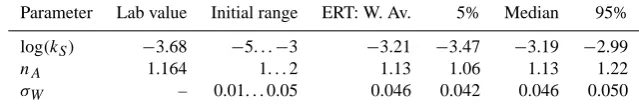
Table 3. Initial and posterior parameter values for the dike and calibration to ERT. Units are m/s forkSand(m)−1forσw.
Parameter Lab value Initial range ERT: W. Av. 5% Median 95%
log(kS) −3.68 −5. . .−3 −3.21 −3.47 −3.19 −2.99
nA 1.164 1. . . 2 1.13 1.06 1.13 1.22
σW – 0.01. . . 0.05 0.046 0.042 0.046 0.050
laboratory measurements. It is clearly visible that as soon as markable changes in water content occur (after 24 h), the filter quickly constrains the parameter range.
The distributions ofα andn in Fig. 7 have hardly been constrained. A strong correlation between these parameters was observed in Huisman et al. (2010), which leads to a very slow convergence as many possible pairs ofαandnprovide acceptable simulations. This is also apparent in Fig. 9. Here, the distribution of particle weights is shown as a function of the parametersn andα. The ridge of the weight land-scape has approximately the same height for a large range of parameter combinations, leading to a slowly converging estimation. In the limited number of time steps of the filter-ing process, no convergence could be achieved, however, the median and weighted average approach the laboratory val-ues. The petrophysical parametersnAandσwhave been well
constrained as shown in Fig. 8. The value ofnAagrees very
well with the estimate ofnA=1.16 by Rings et al. (2008).
A comparison of water content distributions using labora-tory and ERT calibratedkSfor the 2005 experiment att=29 h
is shown in Fig. 10. As the subsurface seen by ERT is limited to a depth of about 1.5 m on the landside (see Rings et al., 2008), ERT starts to detect changes in water content from t=20 h on. At t=29 h, the parameter kS as estimated by
the coupled approach leads to a simulation with mostly es-tablished saturated area (Fig. 10, top row, right). The lower kSas determined in the laboratory, however, leads to a
satu-rated area that would barely reach the region visible to ERT (Fig. 10, top row, left). After t=29 h, a saturated area is established and the measurements seem to carry few infor-mation to additionally constrain the posterior distributions. However, these time steps are important to allow the poste-rior distribution to converge through additional resampling steps.
The RMS error of the modelled ERT response in the last time step is 311m with a variance of only 16m. This is twice the RMSE as found by the MCMC optimization in Huisman et al. (2010), which had 12 free parameters, but a significant reduction from the initial RMS of 1966m with a variance of 989m. From the small variance of the RMSE in the final set of particles, it is concluded that the filter has approximately converged to the posterior distribution that re-flects the uncertainty and information content of the mea-surements.
To evaluate the influence of the number of particles, we repeated the ERT filter run with only 400 particles. While the constraints on the parameter distributions look similar to those in Fig. 8 with only slightly wider bounds, the median and weighted averages differ considerably between runs with 400 and 4096 particles. Figure 11 shows the particle weight distributions in thekS parameter space at timet=78 h. The
[image:8.595.135.455.201.255.2]Fig. 7. Posterior probability obtained from TDR measurements.
Distributions of kS, α and nare shown with the 98% percentile
marked by light color, the 50% percentile marked in blue, the blue line marking the median and the green dots marking the weighted averages at each time step. Green diamonds on the axes mark the laboratory values.
5 Conclusions
We have presented a sequential Bayesian framework for es-timation of hydrological states and parameters from hydro-geophysical measurements. This particle filter method ap-proaches the pdfs of state and parameters by discrete sets of particles which each carry state and parameters sampled from initial distributions. Through time propagation and compar-ison to measurement data, the particles are assigned weights according to how well they describe the data. Over time and with the help of a resampling technique, the particles proach the true distributions. Furthermore, the filtering ap-proach has the benefit of providing updated posterior
distri-Fig. 8. Posterior probabilities obtained from ERT measurements.
Distributions ofkS,nAandσware shown with the 98% percentile
marked by light color, the 50% percentile marked in blue, the blue line marking the median and the green dots marking the weighted averages at each time step. Green diamonds on the axes mark the laboratory values.
butions of states and parameters whenever new measurement data become available.
For a synthetic data set simulating lysimeter infiltration monitored by ERT, this method was shown to be able to re-trieve the correct model states and parameters and provide a reasonable estimate of the remaining predictive uncertainty. However, it was also apparent that small errors in the state estimation can strongly affect parameter estimation, which necessitates the use of an increased number of particles.
[image:9.595.79.252.65.456.2]Fig. 9. Particle weights,nandαfor all particles in the filter run calibrated to SWC measurements at the final time step.
Fig. 10. Water content distribution in the dike model at timet=29 h for the 2005 experiment using either the laboratory measuredkSor
the (final)kSestimated from ERT.
model. This model dike allows experiments with temporal changes in water content up to full saturation. It was mon-itored by TDR cables in the dike body that measured soil water content, and by ERT perpendicular to the crest on the land side of the dike. Two particle filter runs were made. In the first run, water content measured with TDR was used as the observation model, while in the second run only ERT measurements were analyzed using the coupled hydrogeo-physical inversion approach. The first filter run estimated three hydrological parameters, while the second estimated kSand two petrophysical parameters. The parameter ranges
were successfully constrained forkS and the petrophysical
parameters. For all parameters, the weighted average of the parameter distributions were in good agreement with values obtained in laboratory measurements and previous studies.
[image:10.595.57.275.243.402.2]The results of this study are encouraging and show that sequential Bayesian methods are an appropriate estimation technique for parameter estimation in hydrogeophysical sur-veys. Even more, as updates of the posterior distributions become available with new measurements, this can be used for on-line parameter estimation in a permanent monitoring
Fig. 11. Particle weights andkS for ERT filter runs with 400 and
4096 particles at tmet=78 h.
installation, e.g. for the continuous monitoring of dike water content. The filter can also be used to forecast future states and to optimize experimental design. This may involve a spa-tial focussing in regions where change will probably occur or an optimization of the timing of measurements in a perma-nently installed system.
Acknowledgements. We thank the reviewers for their constructive
comments. J. Rings thanks the BAW Karlsruhe for the possibility to take measurements on the dike model and A. Scheuermann and A. Bieberstein at the IBF, University of Karlsruhe, for supporting the measurements. J. A. Huisman is supported by grant HU1312/2-1 of the Deutsche Forschungsgemeinschaft.
Edited by: T. Elliot
References
Archie, G. E.: The electrical resitivity log as an aid in determining some reservoir characteristics, American Institute of Mining and Metallurgical Engineers, 55–62, 1942.
Arulampalam, M. S., Maskell, S., Gordon, N., and Clapp, T.: A tutorial on particle filters for online nonlinear/non-Gaussian Bayesian tracking, IEEE T. Signal Proces., 50, 174–188, 2002. Binley, A., Winship, P., West, L. J., Pokar, M., and Middleton, R.:
Seasonal variation of moisture content in unsaturated sandstone inferred from borehole radar and resistivity profiles, J. Hydrol., 267, 160–172, 2002.
Cappe, O., Godsill, S. J., and Moulines, E.: An overview of existing methods and recent advances in sequential Monte Carlo, Proc. IEEE, 95, 899–924, doi:10.1109/JPROC.2007.893250, 2007. Cassiani, G. and Binley, A.: Modeling unsaturated flow in a layered
formation under quasi-steady state conditions using geophysical data constraints, Adv. Water Resour., 28, 467–477, 2005. Chen, J. S., Hubbard, S. S., Rubin, Y., Murray, C., Roden, E., and
Majer, E.: Geochemical characterization using geophysical data and Markov Chain Monte Carlo methods: a case study at the South Oyster bacterial transport site in Virginia, Water Resour. Res., 40, W12412, doi:10.1029/2003WR002883, 2004. Chen, Z.: Bayesian filtering: From Kalman filters to particle filters,
and beyond, Tech. rep., McMaster University, 2003.
Day-Lewis, F. D., Singha, K., and Binley, A. M.: Applying petro-physical models to radar travel time and electrical resistivity to-mograms: resolution-dependent limitations, J. Geophys. Res., 110, B08206, doi:10.1029/2004JB003569, 2005.
Deiana, R., Cassiani, G., Villa, A., Bagliani, A., and Bruno, V.: Cal-ibration of a vadose zone model using water injection monitored by GPR and electrical resistiance tomography, Vadose Zone J., 7, 215–266, 2008.
Douc, R., Cappe, O., and Moulines, E.: Comparison of Resampling Schemes for Particle Filtering, Image and Signal Processing and Analysis, 2005, 64, http://www.citebase.org/abstract?id=oai: arXiv.org:cs/0507025, 2005.
Doucet, A. and de Freitas, N.: Sequential Monte Carlo Methods in Practice, Statistics for Engineering and Information Science, Springer, 2001.
Evensen, G.: Sequential data assimilation with a nonlinear quasi-geostrophic model using Monte Carlo methods to forecast error statistics, J. Geophys. Res., 99, 10143–10162, 1994.
Gordon, N. J., Salmond, D. J., and Smith, A. F. M.: Novel approach to nonlinear/non-Gaussian Bayesian state estimation, IEE Proc.-F, 140, 107–113, 1993.
Hardelauf, H., Javaux, M., Herbst, M., Gottschalk, S., Kasteel, R., Vanderborght, J., and Vereecken, H.: PARSWMS: a parallelized model for simulating three-dimensional water flow and solute
transport in variably saturated soils, Vadose Zone J., 6, 255–259, 2007.
Hendricks Franssen, H. J. and Kinzelbach, W.: Real-time groundwater flow modeling with the ensemble Kalman fil-ter: joint estimation of states and parameters and the fil-ter inbreeding problem, Wafil-ter Resour. Res., 44, W09408, doi:10.1029/2007WR006505, 2008.
Hinnell, A. C., Ferre, T. P. A., Vrugt, J. A., Huisman, J. A., Moysey, S., Rings, J., and Kowalsky, M. B.: Improved extraction of hydrologic information from geophysical data through coupled hydrogeophysical inversion, Water Resour. Res., doi:10.1029/2008WR007060, in press, 2010.
Hsu, K.-L., Moradkhani, H., and Sorooshian, S.: A se-quential Bayesian approach for hydrologic model selec-tion and predicselec-tion, Water Resour. Res., 45, W00B12, doi:10.1029/2008WR006824, 2009.
Hubbard, S. S., Rubin, Y., and Majer, E.: Spatial correlation struc-ture estimation using geophysical and hydrogeological data, Wa-ter Resour. Res., 35, 1809–1825, 1999.
Huisman, J. A., Rings, J., Vrugt, J. A., Sorg, J., and Vereecken, H.: Hydraulic properties of a model dike from coupled Bayesian and multi-criteria hydrogeophysical inversion, J. Hydrol., 38, 62–73, doi:10.1016/j.jhydrol.2009.10.023, 2010.
Jadoon, K. Z., Slob, E., Vanclooster, M., Vereecken, H., and Lam-bot, S.: Uniqueness and stability analysis of hydrogeophysi-cal inversion for time-lapse ground-penetrating radar estimates of shallow soil hydraulic properties, Water Resour. Res., 44, W09421, doi:10.1029/2007WR006639, 2008.
Kaipio, J. and Somersalo, E.: Statistical and Computational Inverse Problems, Springer-Verlag, 2004.
Kalman, R. E.: A new approach to linear filtering and prediction problems, Trans. ASME J. Basic Eng., 82, 35–45, 1960. Kemna, A., Binley, A., Ramirez, A., and Daily, W.: Complex
resis-tivity tomography for environmental applications, Chem. Eng. J., 77, 11–18, 2000.
Kemna, A., Vanderborght, J., Kulessa, B., and Vereecken, H.: Imag-ing and characterisation of subsurface solute transport usImag-ing electrical resistivity tomography (ERT) and equivalent transport models, J. Hydrol., 267, 125–146, 2002.
Kivman, G. A.: Sequential parameter estimation for stochastic sys-tems, Nonlin. Processes Geophys., 10, 253–259, 2003,
http://www.nonlin-processes-geophys.net/10/253/2003/. Koestel, J., Kemna, A., Javaux, M., Binley, A., and Vereecken, H.:
Quantitative imaging of solute transport in a unsaturated and undisturbed soil monolith with 3-D ERT and TDR, Water Re-sour. Res., 44, W12411, doi:10.1029/2007WR006755, 2008. Kowalsky, M. B., Finsterle, S., and Rubin, Y.: Estimating flow
pa-rameter distributions using groundpenetrating radar and hydro-logical measurements during transient flow in the vadose zone, Adv. Water Resour., 27, 583–599, 2004.
Kowalsky, M. B., Finsterle, S., Peterson, J., Hubbard, S., Rubin, Y., Majer, E., Ward, A., and Gee, G.: Estimation of field-scale soil hydraulic and dielectric parameters through joint inversion of GPR and hydrological data, Water Resour. Res., 41, W11425, doi:10.1029/2005WR004237, 2005.
Lehikoinen, A., Finsterle, S., Voutilainen, A., Kowalsky, M. B., and Kaipio, J. P.: Dynamical inversion of geophysical ERT data: state estimation in the vadose zone, Inverse Probl. Sci. En., 1, 1–22, 2009.
Linde, N., Binley, A., Tryggvason, A., Pedersen, L. B., and Revil, A.: Improved hydrogeophysical characterization using joint inversion of cross-hole electrical resistance and ground-penetrating radar traveltime data, Water Resour. Res., 42, W12404, doi:10.1029/2006WR005131, 2006.
Liu, J. and West, M.: Combined Parameter and State Estimation in Simulation-Based Filtering, in: Sequential Monte Carlo Methods in Practice. New York, edited by: Doucet, A., De Freitas, J. F. G., and Gordon, N. J., Springer-Verlag, New York, 2000.
Liu, J. S. and Chen, R.: Sequential Monte Carlo methods for dy-namic systems, J. Am. Stat Assoc., 93, 1032–1044, 1998. Looms, M. C., Binley, A., Jensen, K. H., Nielsen, L., and
Hansen, T. M.: Identifying unsaturated hydraulic parameters us-ing an integrated data fusion approach on cross-borehole geo-physical data, Vadose Zone J., 7, 238–248, 2008.
Moradkhani, H., Hsu, K.-L., Gupta, H., and Sorooshian, S.: Un-certainty assessment of hydrologic model states and parameters: sequential data assimilation using the particle filter, Water Re-sour. Res., 41, W05012, doi:10.1029/2004WR003604, 2005. M¨uller, K., Vanderborght, J., Englert, A., Kemna, A., Rings, J.,
Huisman, J. A., and Vereecken, H.: Imaging and character-ization of solute transport during two tracer tests in a shal-low aquifer using electrical resistivity tomography and multi-level groundwater samplers, Water Resour. Res., 46, W03502, doi:10.1029/2008WR007595, 2010.
Rings, J. and Hauck, C.: Reliability of resistivity quantification for shallow subsurface water processes, J. Appl. Geophys., 68, 404– 416, doi:10.1016/j.jappgeo.2009.03.008, 2009.
Rings, J., Hauck, C., Preko, K., and Scheuermann, A.: Soil water content monitoring on a dike model using electrical resistivity tomography, Near Surf. Geophys., 6, 123–132, 2008.
Rubin, Y. and Hubbard, S. S.: Hydrogeophysics, Water Science and Technology Library, Springer-Verlag Berlin, Heidelberg, New York, 2005.
Rucker, D.: A coupled electrical resistivity-infiltration model for wetting front evaluation, Vadose Zone J., 8, 383–388, doi:10.2136/vzj2008.0080, 2009.
Ruecker, C., Guenther, T., and Spitzer, K.: Three-dimensional mod-elling and inversion of dc resistivity data incorporating topogra-phy – I. Modelling, Geotopogra-phys. J. Int., 166, 494–505, 2006.
Salamon, P. and Feyen, L.: Assessing parameter, precipitation, and predictive uncertainty in a disturbed hydrological model using sequential data assimilation with the particle filter, J. Hydrol., 376, 428–442, 2009.
Scheuermann, A., Huebner, C., Schlaeger, S., Wagner, N., Becker, R., and Bieberstein, A.: Spatial time domain reflectome-try and its application for the measurement of water content dis-tributions along flat ribbon cables in a full-scale levee model, Water Resour. Res., 45, W00D24, doi:10.1029/2008WR007073, 2009.
Schlaeger, S.: A fast TDR-inversion technique for the reconstruc-tion of spatial soil moisture content, Hydrol. Earth Syst. Sci., 9, 481–492, 2005,
http://www.hydrol-earth-syst-sci.net/9/481/2005/.
Sepp¨anen, A., Vauhkonen, M., Vauhkonen, P. J., Somersalo, E., and Kaipio, J. P.: State estimation with fluid dynamical evolution models in process tomography – an application to impedance to-mography, Inverse Probl., 17, 467–483, 2001.
Simunek, J., van Genuchten, M. T., and Sejna, M.: Develop-ment and applications of the HYDRUS and STANMOD software packages and related codes, Vadose Zone J., 7, 587–600, 2008. Storvik, G.: Particle filters for state-space models with the presence
of unknown static parameters, IEEE T. Signal Process., 50, 281– 289, 2002.
Ulrich, C. and Slater, L. D.: Induced polarization measurements on unsaturated, unconsolidated sands, Geophysics, 69, 762–771, 2004.
van Genuchten, M. T.: A closed-form equation for predicting the hydraulic conductivity of unsaturated soils, Soil Sci. Soc. Am. J., 44, 892–898, 1980.
Vereecken, H., Binley, A., Cassiani, G., Revil, A., and Titov, K.: Applied Hydrogeophysics, vol. 71 of IV: Earth and Environmen-tal sciences, NATO Science Series, 2006.
Vrugt, J. A., Diks, C. G. H., Gupta, H. V., Bouten, W., and Ver-straten, J. M.: Improved treatment of uncertainty in hydro-logic modeling: combining the strengths of global optimiza-tion and data assimilaoptimiza-tion, Water Resour. Res., 41, W01017, doi:10.1029/2004WR003059, 2005.
Weerts, A. H. and El Serafy, G. Y. H.: Particle filtering and ensem-ble Kalman filtering for state updating with hydrological con-ceptual rainfall-runoff models, Water Resour. Res., 42, W09403, doi:10.1029/2005WR004093, 2006.