www.hydrol-earth-syst-sci.net/15/841/2011/ doi:10.5194/hess-15-841-2011
© Author(s) 2011. CC Attribution 3.0 License.
Earth System
Sciences
Generalized versus non-generalized neural network model for
multi-lead inflow forecasting at Aswan High Dam
A. El-Shafie1and A. Noureldin2
1Senior Lecturer, Civil and Structural Engineering Dept. University Kebangsaan Malaysia, Malaysia 2Associate Professor, Electrical and Computer Engineering, Royal Military College, Kingston, Canada Received: 24 September 2010 – Published in Hydrol. Earth Syst. Sci. Discuss.: 12 October 2010 Revised: 27 January 2011 – Accepted: 29 January 2011 – Published: 11 March 2011
Abstract. Artificial neural networks (ANN) have been found
efficient, particularly in problems where characteristics of the processes are stochastic and difficult to describe using explicit mathematical models. However, time series predic-tion based on ANN algorithms is fundamentally difficult and faces problems. One of the major shortcomings is the search for the optimal input pattern in order to enhance the forecast-ing capabilities for the output. The second challenge is the over-fitting problem during the training procedure and this occurs when ANN loses its generalization. In this research, autocorrelation and cross correlation analyses are suggested as a method for searching the optimal input pattern. On the other hand, two generalized methods namely, Regular-ized Neural Network (RNN) and Ensemble Neural Network (ENN) models are developed to overcome the drawbacks of classical ANN models. Using Generalized Neural Network (GNN) helped avoid over-fitting of training data which was observed as a limitation of classical ANN models. Real in-flow data collected over the last 130 years at Lake Nasser was used to train, test and validate the proposed model. Re-sults show that the proposed GNN model outperforms non-generalized neural network and conventional auto-regressive models and it could provide accurate inflow forecasting.
1 Introduction
Developing optimal release policies for a multi-objective reservoir such as Lake Nasser is a complex process. Lake Nasser is a vast reservoir in southern Egypt and northern Su-dan. Strictly speaking, “Lake Nasser” refers only to the much larger portion of the lake that is in Egyptian territory (83% of
Correspondence to: A. El-Shafie
the total), with the Sudanese preferring to call their smaller body of water Lake Nubia. The area of Sudan-administered Wadi Halfa Salient was largely flooded by Lake Nasser/Lake Nubia. The lake was created as a result of the construction of the Aswan High Dam across the waters of the Nile between 1958 and 1970. The lake is some 550 km long and 35 km across at its widest point, which is near the Tropic of Cancer. It covers a total surface area of 5250 km2and has a storage capacity of some 157 km3of water.
The complexity is attributed to the explicit stochastic envi-ronment (e.g., uncertainty in future inflows) and the fact that when modelling such environments with high uncertainty, future returns cannot be predicted with acceptable accuracy. In this context, several forecasting models were developed using the univariate auto-regressive moving average repre-sentative of the natural inflow at Aswan High Dam (AHD) (see Fig. 1) (Georgakakos et al., 1995; Georgakakos, 2007). These models tend to either overestimate low flows or un-derestimate high flows. The drawbacks are very significant when it comes to efficient and effective reservoir regulation. Therefore, it is essential to develop a forecasting model that is robust and free from these drawbacks.
River flow is believed to be highly nonlinear, time-varying, spatially distributed and not easily described by simple mod-els. Two major approaches for modelling the river flow forecasting process have been explored in the literature. These are the conceptual (physical) models and the system-theoretic models. Conceptual river flow forecasting mod-els are designed to approximate within their structures (in some physically realistic manner) the general internal sub-processes and physical mechanisms, which govern the hy-drologic cycle. These models usually incorporate simpli-fied forms of physical laws and are generally nonlinear, time-invariant and deterministic, with parameters that are representative of river flow characteristics. Until recently, for practical reasons (data availability, calibration problems,
36
Fig. (1). Location of Aswan High Dam Fig. 1. Location of Aswan High Dam.
etc.) most conceptual river flow-forecasting model assumed combine representations of the parameters. While such mod-els ignore the spatially distributed, time-varying and stochas-tic properties of the river flow process, they attempt to incor-porate realistic representations of the major nonlinearity in-herent in the river flow and climatic parameters relationships. Conceptual river flow models are generally reported to be re-liable in forecasting the most important features of the hydro-graph, such as the beginning of the rising limb, the time and the height of the peak and volume of flow. However, the im-plementation and calibration of such a model can typically encounter various difficulties including sophisticated math-ematical tools, significant amounts of calibration and some degree of experience with the model.
While conceptual models are important in the understand-ing of hydrologic processes, there are many practical situa-tions such as river flow forecasting where the main concern is making accurate predictions at specific locations. In such a situation, it is preferable to develop and implement a sim-pler system-theoretic model instead of developing a concep-tual model. In the system-theoretic approach, models based on differential equations (or difference equations in case of discrete-time systems) are used to identify a direct mapping between the inputs and outputs without detailed considera-tion of the internal structure of the physical processes. The linear time-series models such as ARMAX (Auto Regressive Moving Average with exogenous inputs) models developed by Box and Jenkins (1970) have usually been used in such situations because they are relatively easy to develop and implement. They have been determined in providing satis-factory predictions in many applications (Salas et al., 1980; Wood, 1980; Bras and Rodriguez-Iturbe, 1985). However, such models do not attempt to represent the nonlinear dy-namics inherent in the river streamflow and, therefore, may not always perform adequately.
Motivated by the difficulties associated with nonlinear models, their complex structure and parameter estimation
techniques, some truly nonlinear system-theoretic river flow forecasting models have been reported. In most cases, lin-earity or piece-wise linlin-earity has been assumed (Natale and Todini, 1976). Allowing the model parameters to vary with time can compensate for the model structural errors that may exist. For example, real-time identification techniques, such as recursive least squares and state-space Kalman filtering, have been applied for adaptive estimation of model param-eters (Chiu, 1978; Kitanidis and Bras, 1980a, b; Bras and Rodriguez-Iturbe, 1985).
The success with which Artificial Neural Network ANNs have been used to model dynamic systems in several fields of science and engineering suggests that the ANN approach may prove to be an effective and efficient way to model the river flow process in situations where explicit knowledge of the internal hydrologic sub-process is not available. Some studies in which ANN models have been applied to problems involving river watershed and weather prediction have been reported in the literature. Kang et al. (1993) developed ANNs for daily and hourly streamflow forecasting based on the his-torical inflow data at the same incremental rate (daily and/or hourly) using one of four pre-specified network structures. Seno et al. (2003) proposed a new model architecture for in-flow forecasting of the Karogawa Dam utilizing not only the rain data inside the dam basin, but also the outside rain data. The proposed architecture reduced the overall inflow fore-casting error by about 30%. Coulibaly et al. (1998, 1999, 2000 and 2001) introduced several ANN inflow-forecasting models with different neural network types and various input data structures. It was reported that recurrent neural networks (RNN) can be appropriately utilized for inflow forecasting while taking into consideration the precipitation, snowmelt and temperature. However, it was also reported that a com-plex training procedure, as well as long training time, is re-quired in order to achieve the desired performance.
made their contributions in the rainfall-runoff calibrations and Chau (2006), Lin et al. (2006), Wang et al. (2009)and Wu et al. (2009) in flow forecasting, utilizing different meth-ods of optimization by genetic algorithm and particle swarm optimization.
Recently, the authors already developed Artificial Intel-ligent (AI) model for inflow forecasting at AHD utilizing Adaptive Neuro-Fuzzy Inference System (ANFIS), Mutli-Layer Perceptron Neural Network MLPNN and Radial Basis Function Neural Network (RBFNN), (El-Shafie et al., 2007, 2008, 2009). In fact, those models showed very good po-tential for providing a relatively high level of accuracy for inflow forecasting at AHD. Obviously, AI provides a viable and effective approach for developing input-output forecast-ing models in situations that do not require modellforecast-ing of the whole and/or part of the internal parameter of the river flow. Although, those models have proved to be efficient, its con-vergence tends to be very slow and yields sub-optimal solu-tions. This may not be suitable for dynamic adaptive accurate forecasting purpose. In fact, the major objective of training an ANN for prediction is to generalize, i.e., to have the out-puts of the network approximate target values given inout-puts that were not in the training set. However, time series pre-diction based on ANN learning algorithms is fundamentally difficult and faces problems. One of the major shortcomings is that the ANN model experienced an over-fitting problem while in a training session and occurs when a neural network loses its generalization.
The aim of this paper is to introduce two generalization methods to be integrated with classical MLPNN to overcome the over-fitting problem. Among different types of neural networks, this research focuses mainly on MLPNN for pre-diction, because of the inherent simple architecture of these networks. However, any other neural network architecture will be acceptable through this approach. These methods are suitable for the application of predicting time series of com-plex systems’ behaviour, based on neural networks and us-ing soft computus-ing methods. The main idea of the proposed method is to introduce a technique to overcome the over-fitting problem while developing ANN prediction model. Fi-nally, the proposed methods will be examined and compared with the developed non-generalized MLPNN for inflow fore-casting at AHD.
2 Data collection and analysis
In this study, the Nile River inflow data in Aswan published by the Egyptian Ministry of Water Resources and Irrigation was utilized. The inflows in Aswan for the period between 1871 and 1902 have been deduced using a general stage-discharge table, which has been constructed from the Aswan downstream gauge. Due to the construction of several dams and other hydraulic structures in Egypt and Sudan, the natu-ral inflow from 1902 onwards has been derived directly from
the general stage-discharge relationship in Aswan by cor-recting the measured inflow from the effect of losses from upstream reservoirs, abstractions in Sudan and the effect of regulation by Sennar Reservoir.
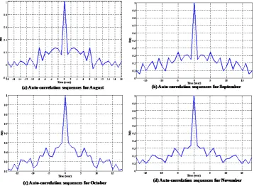
From the data collected, it is obvious that the natural in-flow is random in nature. Accordingly, it is recommended to analyse the data by studying the auto-correlation sequences for each month over the 130 years and the cross-correlation between consequent months in the same year. The study of the auto-correlation function clearly tells how the process is correlated with itself over time. While studying the cross-correlation sequences, it provides information about the mu-tual correlation between two consequent months.
The auto-correlation sequence for a random processx(t ), corresponding to a monitored inflow at a certain month, is defined as
Rx(t )(τ )=
E ((xt −µ)(xt+τ−µ))
σ2 (1)
Whereτ is the independent time variable of the autocorrela-tion sequenceR (τ ),µis the expected value ofXtandσ its variance.
On the other hand, the cross-correlation sequence between the processesx(t )andy(t ), corresponding to inflows at two consequent months, is defined as
Rx(t ),y(t )(τ )=
E ((xt −µ)(yt−µ)) σxσy
(2) Figure 2 shows the auto-correlation sequence for 4 different months with respect to time over 130 years. Obviously, these auto-correlation sequences decrease rapidly with respect to time showing insufficient correlation over time. In this case, the auto-correlation function is more likely to represent a white sequence which is impossible to predict over time. In other words, it is unlikely to use neural networks to predict the inflow of a certain month at a certain year utilizing the monitored/forecasted inflow of the same month from previ-ous years.
Fortunately, studying the cross-correlation between the in-flow at montht(Q(t)) and the inflow at three previous months (Q(t−1), Q(t−2), Q(t−3)) showed a strong correlation over time. Figure 3 shows the cross-correlation function between August and the previous three months (July–June– May).
3 Methodology
3.1 Artificial Neural Network and over-fitting
Artificial Neural Networks (ANN) is densely interconnected processing units that utilize parallel computation algorithms. The basic advantage of ANN is that they can learn from rep-resentative examples without providing special programming modules to simulate special patterns in the dataset (Gibson
37
Fig. (2). The auto-correlation sequence for the inflow for months of
Fig. 2. The auto-correlation sequence for the inflow for months of(August, September, October, November).
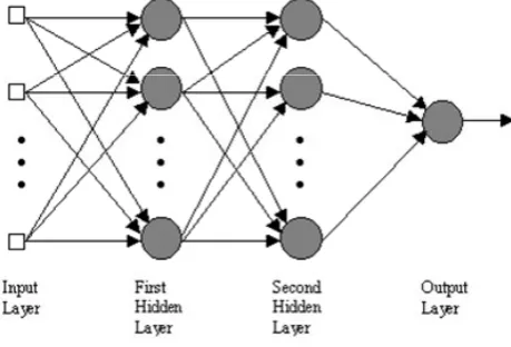
and Cowan, 1990). This allows ANN to learn and adapt to a continuously changing environment. Therefore, ANN can be trained to perform a particular function by tuning the values of the weights (connections) between these elements. The training procedure of ANN is performed so that a particular input leads to a certain target output as shown in Fig. 4.
The input and output layers of any network have numbers of neurons equal to the number of the inputs and outputs of the system, respectively. The architecture of a multi-layer feed-forward neural network can have many layers between the input and the output layers where a layer represents a set of parallel processing units (or nodes), namely the hid-den layer. The main function of the hidhid-den layer is to allow the network to detect and capture the relevant patterns in the data and to perform complex nonlinear mapping between the input and the output variables. The sole role of the input layer of nodes is to relate the external inputs to the neurons of the hidden layer. Hence, the number of input nodes corre-sponds to the number of input variables. The outputs of the hidden layer are passed to the last (or output) layer, which provides the final output of the network. Finding a parsimo-nious model for accurate prediction is particularly critical, since there is no formal method for determining the appro-priate number of hidden nodes prior to training. Therefore, here we resort to a trial-and-error method commonly used for network design.
One of the most important aspects of machine learning models is how well the model generalizes to unseen data. The over-fitting problem occurs when a neural network loses
its generalization feature. In other words, it cannot gener-alize the relations which exist between training inputs and their related outputs to the similar hidden patterns of the un-observed data. In such cases the performance of neural net-work measured on the training set is much better compared to new inputs. In predicting time series, the aim is to be able to deal with time varying sequences. This can be achieved if the network input-output patterns involved in such a way that it can respond to temporal sequences. Consequently, net-works within its structure should be considered as a good choice. However, whatever architecture is used, some defi-nite problems such as over-fitting will be met (Tetko et al., 1995; Haykin, 1994; Bishop, 1996; Duda et al., 2001; Box and Jenkins, 1970).
In the following section, a brief description for ANN model for inflow forecasting at AHD will be reported (El-Shafie et al., 2008), then the proposed methods for gener-alization will be applied to overcome the experienced over-fitting in the model.
3.2 Inflow forecasting with Multi-Layer Perceptron
(MLP) Neural Network
38
Fig. (3). The cross-correlation sequence for the inflow for months of
[image:5.595.312.542.376.532.2]* C.C.S. (t) represents the cross correlation sequence of the two variables (Brown and Hawng 1997)
Fig. 3. The cross-correlation sequence for the inflow for months of (August–July, August–June, August–May). ∗C.C.S. (t) represents the cross-correlation sequence of the two variables (Brown and Hawng, 1997).
hidden layer becomes a well-conditioned result of the total system behaviour and then the prediction can be done after this stage.
Comprehensive data analysis for the historical inflow pat-tern for each month has been carried out (El-Shafie et al., 2008). In fact, the monitored inflow is random in nature and has to be modelled stochastically in order to develop an ap-propriate inflow forecasting method. Stochastic models are always established based on correlation analysis (El-Shafie et al., 2008). Accordingly, an analysis of such random in-flow data by studying the auto-correlation sequences for each month over the past 130 years and the cross-correlation be-tween consecutive months in the same year was performed (El-Shafie et al., 2008). The study of the auto-correlation function clearly informs us how the process is correlated with itself over time and, while studying the cross-correlation se-quences, provides information about the mutual correlation between two consecutive months. Such analyses allow for the achievement of the appropriate number of inflows of the prior months utilized as input to the ANN model in order to provide accurate inflow forecasting at a certain month. More-over, the inflow forecasted at montht can be used with the monitored inflow of some previous months to provide a fore-casting at month t+1. This procedure of using the fore-casted inflow can be repeated forL months with the value ofL dependent upon the environmental conditions and the basin characteristics (Salem and Dorrah, 1982). It has been reported by Atiya et al. (1990) that the lead-timeLcannot be more than three months.
39
Fig. (4). Artificial Neural Network Model DiagramFig. 4. Artificial neural network model diagram.
Our pilot investigation showed that inflow forecasting at month t, based on the monitored inflow from the previ-ous years of the same month (instead of previprevi-ous months of the same year), cannot provide reliable results. There-fore, in this study, ANN, with its nonlinear and stochastic modelling capabilities, is utilized to develop a forecasting model that mimics the inflow pattern at AHD and predicts the inflow pattern for three months ahead based upon the monitored/forecasted inflow from the three previous months (El-Shafie et al, 2008). The inflowQfforecasted at month t, based on the inflow monitored Qmat the previous three
40
Train NN Q(t+1)
Mean Square Error < 10-4
Adjust weight using scaled conjugate
gradient
Save NN for Q(t+1)
Repeat for all t
t= month
Save 12 NN Input Data Inflow Q(t), Q(t-1) and Q(t-2)
Start Multi-Lead forecasting
Input Data Inflow Q(t), Q(t-1) and Q(t-2)
Call NN (Q(t+1))
Forecast for (Q(t+1))
Input Data Forecasted Q(t+1), Q(t) and Q(t-1)
Call NN (Q(t+2))
Forecast for (Q(t+2))
Input Data
Forecasted Q(t+2), forecasted Q(t+1) and Q(t)
Call NN (Q(t+3))
Forecast for (Q(t+3))
End
No
[image:6.595.116.481.65.326.2]yes
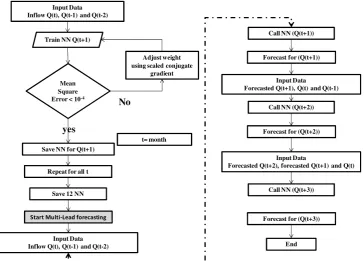
Fig. (5). Schematic representation of the proposed inflow forecasting procedure
Fig. 5. Schematic representation of the proposed inflow forecasting procedure.
months, can be expressed as:
Qf(t )=f (Qm(t−1),Qm(t−2),Qm(t−3)) (3) Consequently, the inflow for montht+1 can be forecasted as follows:
Qf(t+1)=f (Qm(t−1),Qm(t−2),Qm(t−3)) (4) Qf(t+1)=f (Qf(t ),Qm(t−1),Qm(t−2)) (5) Similarly, the inflow for montht+2 can be forecasted using the following equations:
Qf(t+2)=f (Qm(t−1),Qm(t−2),Qm(t−3)) (6) Qf(t+2)=f (Qf(t+1),Qf(t ),Qm(t−1)) (7) Qf in all of the above equations represents forecasted in-flow while Qm is a monitored inflow. It should be noted that Eqs. (4) and (6) introduced the procedure of the first ap-proach, while Eqs. (5) and (7) represent the procedure for the second approach proposed for multi-lead forecasting. A schematic representation of the above procedure is given in Fig. 5. However, an examination for the forecasting skills utilizing different input pattern will be carried out in order to evaluate and verify the findings of the cross-correlation anal-ysis. With the purpose of performing the multi-lead forecast-ing, two approaches have been carried out. The first approach is to useQm(t−1),Qm(t−2) andQm(t−3) to predict the in-flow onQ(t+1), in other word, is to rely only on the natural
inflow as presented in Eqs. (2a) and (3a). While the second approach is to utilize forecasted inflow atQ(t) (Qf(t)) even it has a certain level of error, but at the same time highly correlated with output, Qm(t−2) andQm(t−3) to predict Q(t+1).
The ANN model is established using the above three equations. The architecture of the network consists of an input layer of three neurons (corresponding to the moni-tored/forecasted inflow of the previous three months at the inputs to the network), an output layer of one neuron (corre-sponding to the forecasted inflow) and a number of hidden layers of arbitrary number of neurons at each layer. In order to achieve the desirable forecasting accuracy, twelve ANN architectures were developed (one for each month). Monthly natural inflows for the period of sixty years, from 1871 to 1930, were utilized in order to train the twelve networks. The performance and the reliability of the ANN models were ex-amined using the inflow data monitored between 1931 and 1960. The capabilities of the developed ANN models were further verified by the inflow data between 1961 and 2000, which corresponds to the inflow monitored after the con-struction of AHD in 1960.
41 Hidden Layer I with
6 neurons
Output Layer With one neuron Input Layer
with three neurons
Inflow at month (t)
Inflow at month (t-1)
Inflow at month (t-2)
Inflow at month (t+1)
Neuron
Hidden Layer II with 4 neurons
[image:7.595.119.477.65.278.2]Hidden Layer III with 2 neurons
Fig. (6). The Neural Network Architecture for August
Fig. 6. The neural network architecture for August.
network. There is, however, some practical limits which should generally not be exceeded. According to Caudill (1991) a single hidden layer is usually sufficient unless there is an overriding, truly completing need to go to three hidden layers. Such recommendations arose from the fact that the back-propagation learning rule used to train the network may become ineffective when dealing with such multi-layered networks. As the number of hidden layers increases, the sur-rogate metric used to quantify necessary changes in the in-ternal knowledge representation loses its theoretical ground-ing. On the other hand, the method currently available to determine the correct number of neurons in the hidden lay-ers is experimentation. In the experimentation process, net-works with different numbers of hidden neurons are trained and evaluated for their ability to generalize and detect signif-icant input features. The network with the least number of neurons that is still able to detect all significant features is considered as the network with the optimal number of neu-rons. In this context, in this study, the maximum number of the neuron within each hidden layer is two times the number of input neuron in the input layer.
[image:7.595.310.547.341.494.2]In this study, the choice of the number of hidden layers and the number of neurons in each layer is based on two per-formance indices. The first index is the root-mean-square (RMS) value of the prediction error and the second index is the value of the maximum error. Both indices were obtained while examining the ANN model with the inflow data be-tween 1931 and 1960. The last group of data (bebe-tween 1961 and 2000), that was not used in training, was used to ver-ify the capabilities of the ANN model. An example of ANN architecture used for predicting the inflow for the month of August is presented in Fig. 6 (El-Shafie et al., 2008).
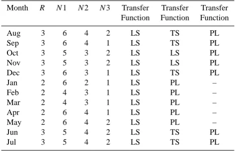
Table 1. The ANN architecture for each month.
Month R N1 N2 N3 Transfer Transfer Transfer
Function Function Function
Aug 3 6 4 2 LS TS PL
Sep 3 6 4 1 LS TS PL
Oct 3 5 3 2 LS LS PL
Nov 3 5 3 2 LS LS PL
Dec 3 6 3 1 LS TS PL
Jan 2 6 2 1 LS PL –
Feb 2 4 3 1 LS PL –
Mar 2 4 3 1 LS PL –
Apr 2 6 4 1 LS PL –
May 2 6 4 2 LS PL –
Jun 3 5 4 2 LS TS PL
Jul 3 5 4 2 LS TS PL
R: Number of hidden layers
N(i): number of neuron in the Hidden layer (i) LS: Log sigmoid
TS: Tan sigmoid PL: Pure-line
The number of hidden layers (R)and the number of neu-rons in each layer (N )for twelve networks are presented in Table 1. The transfer functions used in each layer of the net-works are also listed in Table 1. All twelve netnet-works utilize the backpropagation algorithm during the training procedure. Once the network weights and biases are initialized, during the training process the weights and biases of the network are iteratively adjusted to minimize the network performance function mean-square-error MSE – the average squared er-ror between the network outputs a and the target outputs t. In order to overcome and improve the proposed model performance, two procedures are introduced hereafter in the following sub-sections.
Over-fitting has often been addressed using techniques such as weight decay, weight elimination and early stop-ping to control over-fitting (Weigend et al., 1992). Among these methods Early-stopping is the most well-known solu-tion (Prechelt, 1998). However, using this method on time series of complex systems’ behaviour, it stops the training process too early and the chance of detecting meaningful re-lations between the network outputs and actual behaviour of the complex system does decrease. This indicates that the resulting model will not have proper features for predicting the time series of the system’s behaviour. In the proposed method, we do not focus on removing the over-fitting prob-lem for a single neural network. Instead the major effort is to find an algorithm which is applied on the outputs of the over-fitted networks to produce the correct results. This algorithm will be presented in the following sections.
3.3 Neural network generalization
3.3.1 Regularization procedure
Network over-fitting is a classical machine learning prob-lem that has been investigated by many researchers (Schaffer, 1993; Stallard and Taylor, 1999). Network over-fitting usu-ally occurs when the network captures the internal local pat-terns of the training dataset rather than recognizing the global patterns of the datasets. The knowledge rule-base that is ex-tracted from the training dataset is, therefore, not general. As a consequence, it is important to recognize that the specifica-tion of the training samples is a critical factor in producing a neural network capable of making the correct responses. The problem of over-fitting has also been investigated by re-searchers with respect to network complexity (Ripley, 1996; Ooyen and Nienhuis, 1992; Livingstone, 1997).
Here, to avoid an over-fitting problem, we utilized the regularization technique (Nordstr¨om and Svensson, 1992). This is known as a suitable technique when the scaled con-jugate gradient descent method is adopted for training, as is the case in this study. The regularization technique involves modifying the performance function which is normally cho-sen to be the sum of squares of the network errors on the training set defined as:
MSE=1
2 n X
P=1
(YO−YP)2 (8)
The modified performance function is defined by adding a term that consists of the mean of the sum of squares of the network weights and biases to the original mean-square-error (MSE) function as:
MSEreg=γ ×MSE+(1−γ )×MSW (9) Whereγ is the performance ratio that takes values between 0 and 1; and MSW is computed as:
MSW= 1
M M X
j=1
wj2 (10)
whereM is the number of weights utilized inside the net-work structure and w is weight matrix of the netnet-work. Using the performance function of Eq. (8), the neural networks to predict the inflow at AHD were developed with the intention to avoid over-fitting of data.
3.3.2 Assembly Neural Network Procedure
Initialization phase
In this procedure, it is proposed that in finding a technique based on ensemble neural networks (Chiewchanwattana et al., 2002; Drucker et al., 1994; Cheni et al., 2005), using over-fitted neural networks leads to generalization. In order to achieve this goal, we use a sequence of the previous sys-tem behaviour as the training data, then generate a sequence of inputs with the proper length and their corresponding out-puts from first, the 90 percent of 60 years (training data) and then with respect to the size of the best period from the previ-ous section. Subsequently, we construct a series of networks by guessing the number of hidden layers’ neurons and initial-ize their parameters randomly. Finally, for every network, the parameters vector will stop on a local minimum of its perfor-mance surface. Up to this point, all of the networks are over-fitted on the training set. Afterwards, a Simulated Annealing process is applied on each network. To do this, the model is modified to generate a set of vectors named the noise vec-tors. The length of each noise vector is equal to the length of each network parameters vector and its components are random numbers with uniform distribution between −0.05 and +0.05. By adding noise vectors to the network param-eter vectors, a new set of network paramparam-eters are obtained. This action makes relatively minor changes to the location of each network in its state space.
Networks are trained with these noisy parameters until an-other local minimum is achieved. Making noise vectors and training are repeated for a number of times and the outputs of these networks are compared to the following 10 percent of the 60 years which are not used during training steps. The winner has the best generalization amongst all and is selected as the first member of an ensemble of neural networks.
Learning phase
In this phase, a random vector of lengthNis generated where N is the length of the sequence of the first 60 years of time series values. This vector is called data noise vector and is shown by the following equation:
42 Add New Best Net to
the Ensemble
End
Compute New n1,n2 Values for each layer and new noise values
Create a new set of K networks with n1,n2 neurons in layers
Train the networks with input Data
Simulate these set of networks e2 = prediction error
on Test Data Test the nets with test Data and
choose the best net
Simulate these set of networks e1 = prediction error
on Test Data
[image:9.595.113.480.68.363.2]Noise New Best Net Input Data Test Data Test Data Neural Network Ensemble e1>e2 Terminatio n Condition
+
T F F T+
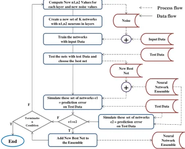
Neural Network Ensemble Process flow Data flowFig. (7). Learning Phase Process for Ensemble Neural network
Fig. 7. Learning phase process for ensemble neural network.
+0.05. Also, M = Max–Min where Max and Min are the maximum and minimum values of time series of the sys-tem’s behaviour, respectively. Once again, we select the net-work that has the best generalization on these new training datasets. But this time, the number of neurons in the hidden layers of networks is calculated using the following equa-tions:
n01=
x×n1
n2 (12)
n02=x+n2 (13)
Wheren1andn2are the initial number of neurons in the first and second hidden layers of the first set of networks andn01 andn02are new values. The value ofxis gained through the following equation: x=
IN+1 2
×mod((IN−1),2) (14) − ("
IN+1 2 ×
1+sign( n2−
IN+1 2 2 +
(2×n2−
IN+1 2
)−1 ×
1−sign( n2−
IN+1 2 2 +0.5 # ×mod(IN,2) )
In this equation, IN is the iteration number. Following the initial step, if IN is even the networks will be constructed with the previous structure, but with more neurons. However, if IN is odd then the number of neurons will be decreased un-til a zero limit is met. At this step, we will continue the pro-cess by increasing the number of neurons. This enables us to find more suitable number of neurons in the completion pro-cess of the ensemble if the initial guess was not accurate and networks need more (or less) number of neurons to achieve a good generalization.
After finding the best network in each set, we compute the sum of absolute errors in the prediction of the last 10 percent of data using the following equations:
e1= z P
i=1 k P
j=1
|Ts(j )−Pr(i,j )|
z (15)
e2=
z+1 P
i=1 k P
j=1
|Ts(j )−Pr(i,j )|
z+1 (16)
In the above equationszis the number of networks that was added to the ensemble before this step. Ts is the sequence of the last 10 percent events of time series in training dataset andkis the size ofTs. Pr(i,j )is the value thatithmember
43
0 10 20 30 40 50 60 70
10-4 10-3 10-2 10-1 100
# Epochs
M
ea
n
S
q
u
a
re
E
rr
o
r
(M
S
E
)
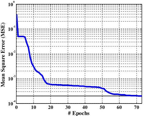
Fig. (8). Training Curve for August
Fig. 8. Training curve for August.
of ensemble predicts for thejthevent in the last 10 percent of time series events. If e1> e2, adding the best network of this step to the ensemble has caused improvements in the generalization of the ensemble totally. Otherwise, we do not add the selected network to the ensemble and repeat this step again with new noisy datasets and a new set of networks with different number of neurons in their hidden layers. The ter-minating condition is as follows: a predefined number of it-erations (namelyitr)are considered and at the end of these iterations the improvement of ensemble predictions (on the last 10 percent) are measured. If this value is smaller than a predefined factor, the termination condition is met. Oth-erwise this process will be repeated. Figure 7 illustrates the learning phase for the proposed ensemble ANN model.
4 Results and discussions
The ANN model architecture of Fig. 5 is employed in this study to provide inflow forecasting for each month. The monitored inflow over sixty years between 1871 and 1930 was used to train twelve networks with each network cor-responding to one month. All twelve networks successfully achieved the target MSE of 0.0001. For example, the train-ing curve for the month of August is demonstrated in Fig. 10 showing convergence to the target MSE after 73 iterations. Two sets of analysis were performed: network without gen-eralization and network with gengen-eralization.
However, evaluation for the ANN model performance has been developed utilizing different input patterns rang-ing between one input (Q(t−1)) and five input (Q(t−1), Q(t−2),. . . , Q(t−5)). Figure 9 shows the best RMSE (BCM) achieved for each input pattern. It could be observed from Fig. 9 that the RMSE values efficiently improved when using three inputs over the RMSE values when using one
44
0.00 0.20 0.40 0.60 0.80 1.00 1.20 1.40 1.60
Aug Sep Oct Nov Dec Jan Feb Mar Apr May Jun Jul
R
o
o
t
M
ea
n
S
q
u
a
re
E
rr
o
r
(R
M
S
E
)
B
C
M
Month
One input
Two input
Three input
Four input
[image:10.595.50.287.63.253.2]Five input
Fig. (9). Root Mean Square Error (BCM) for different input pattern during the period between 1931 and 1960
Fig. 9. Root Mean Square Error (BCM) for different input pattern
during the period between 1931 and 1960.
and two inputs for all months with the exception of August, September and October. This is due to the fact that these three months are the wettest months of the year. On the other hand, the RMSE values increased for all the months once in-cluding more inputs in the input layer. In order to keep the model input pattern consistent for all months, it was decided to consider the previous three months natural inflow as the input pattern.
[image:10.595.314.544.64.214.2]45
(a)
[image:11.595.118.481.64.325.2](b) (c)
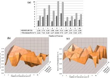
Fig. (10). Neural Network Performance “RMSE and maximum error%” utilizing different Architecture, (a) one hidden layer (b) & (c) two hidden layers
Fig. 10. Neural Network Performance “RMSE and maximum error%” utilizing different Architecture, (a) one hidden layer (b) and (c) two
hidden layers.
the summation of the error distribution within the validation period is not high. Consequently, by using both indices it guarantees the consistent level of errors by providing a great potential for having the same level error while examining the model for unseen data in the testing period.
In order to show how the trial and error procedure for se-lecting the best parameter set of certain ANN architecture was performed, an example for the month of January is pre-sented in Fig. 10. For better visualization, the inverse value of both RMSE and maximum error were used as seen in Fig. 10b and c instead of the real values, while Fig. 10a shows the real value for both indices. Figure 10 shows the changes in the value of the RMSE and the maximum error versus the number of neurons when the number of hidden layers is one (Fig. 10a) and for two hidden layers in Fig. 10b (RMSE) and c for the maximum error during the validation period between 1930 and 1960. It is interesting to observe the large number of local minima that exist in both domains. It can be observed that the best combination of the proposed statistical indices for evaluating the forecasting model for the month of January when the ANN architecture has 6 neurons in the first layer and 2 neurons in the second layer, achieving RMSE 0.65BCM and maximum error 2.92%.
The optimal number of hidden layers (R) and the number of neurons in each layer (N) for twelve networks are pre-sented in Table 1. The transfer functions used in each layer of the networks are also listed in Table 1. All twelve net-works utilize the backpropagation algorithm during the
train-ing procedure. Once the network weights and biases are ini-tialized during the training process, the weights and biases of the network are iteratively adjusted to minimize the network performance function mean square error (MSE) – the average squared error between the network outputsa and the target outputst. In order to overcome and improve the proposed model performance, two procedures are introduced hereafter in the following subsections.
4.1 Non-generalized network
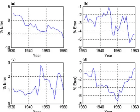
The twelve non-regularized networks developed during the training procedure are used to provide the inflow forecast-ing for the next thirty years between 1931 and 1960. Since the inflow was accurately monitored over the thirty year pe-riod, the performance of the proposed ANN-based architec-ture can be examined and evaluated. The distribution of the percentage value of the error over these thirty years, as well as its RMS value, are the two statistical performance indices used to evaluate the model accuracy. The distribution of the percentage error between the monitored (actual) and the fore-casted inflows for four different months over thirty years be-tween 1931 and 1960 is shown in (Fig. 11). It can be ob-served that the highest percentage error for these four spe-cific months is 7%. However, other months (October, April, May and July) show higher percentage errors, up to 18%, as depicted in (Fig. 12).
46
(a) (b)
(c) (d)
Fig. (11). Error distribution for (a) August (b) December (c) January (d) June
Fig. 11. Error distribution for (a) August (b) December (c) January (d) June.
Table 2 shows the RMS value of the error over the same thirty years for the different months. Small RMS values of the errors associated with the months of (August, Septem-ber, November and March) can be observed. This agrees with the relatively small percentage errors shown in (Fig. 11). Although, the RMS values of the errors associated with the months of February and May might look small, they corre-spond to relatively small values of the monitored inflow. For example, RMS error values of 1.0689 Billion Cubic Meter (BCM) and 0.2282 BCM have been evaluated for the months of October and February, respectively. These values of RMS errors are relatively high since they correspond to monitored inflow range of 27.40–5.97 BCM for October and 6.04–1.15 BCM for February. On the other hand, RMS error values of 0.49 BCM and 0.0909 BCM have been evaluated for the months of August and March, respectively. These values of RMS errors are relatively small as they correspond to moni-tored inflow range of 29.10–6.50 BCM for August and 5.81– 1.07 BCM for March, respectively.
In the search for a better understanding of the above ob-servations, further analysis was performed to study the re-lation between the root-mean-square error (RMSE) and the average monitored inflow associated with each month. The analysis was carried out through scaling the errors by divid-ing the RMSE values by the average monitored inflows over the period between 1871 and 1930 for each month, see Ta-ble 2, Column 5. It becomes obvious that the non-regularized ANN models require further optimization to produce robust forecasting with consistent error levels over all networks. The problem of non-consistent prediction is always related to over-fitting during learning (Ripley, 1996; Haykin, 1999). The over-fitting problem is simply that the network was only trained to memorize the training examples and it did not learn to generalize.
47
(a) (b)
(c) (d)
Fig. (12). Error Distribution for (a) October (b) April (c) May (d) July
Fig. 12. Error Distribution for (a) October (b) April (c) May
[image:12.595.53.285.61.247.2](d) July.
Table 2. RMSE associated with NN forecasting model for each
month.
Month RMSE Maximum Minimum RMSE/
(BCM) inflow (BCM) inflow (BCM) (Ave Inflow)
Aug 0.4900 29.10 6.50 0.0275
Sep 0.7805 32.79 7.31 0.0389
Oct 1.0689 27.40 5.97 0.0640
Nov 0.1801 14.40 4.12 0.0194
Dec 0.2838 11.00 2.83 0.0410
Jan 0.2347 7.70 1.72 0.0490
Feb 0.2282 6.04 1.15 0.0634
Mar 0.0909 5.81 1.07 0.0264
Apr 0.2389 5.26 0.95 0.0760
May 0.3215 4.72 0.80 0.1164
Jun 0.2665 5.16 0.90 0.0879
Jul 0.5544 11.03 1.74 0.0868
4.2 Generalization of Neural Network
[image:12.595.309.547.65.244.2] [image:12.595.309.548.342.494.2]48
(a) (b)
(c) (d)
Fig. (13). Error Distribution after Regularization for (a) October (b) April (c) May (d) July
Fig. 13. Error Distribution after Regularization for (a) October (b) April (c) May (d) July.
can be determined that the regularized network improved the distribution of errors by about 40% for October compared with non-regularized network.
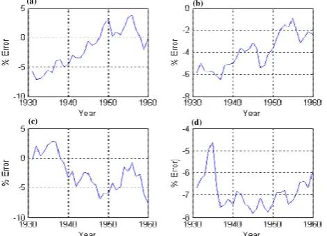
On the other hand, the ensemble ANN model is applied to the same four months (October, April, May and July) which experienced over-fitting problem while training. Figure 14 shows that 4, 8, 10 and 5 networks are selected as ensem-ble members for the above-mentioned months, respectively, before the termination conditions met. It should be noted that the RMSE calculated here is associated with the last 10 percent (1924–1930) of the training dataset between 1871 and 1930. Utilizing ensemble ANN method, as shown in this figure, could reduce the RMSE significantly if compared with the non-generalized ANN method (over-fitted network). Moreover, the performance of the ensemble ANN model dur-ing the testdur-ing data period between 1930 and 1960 was exam-ined. Figure 15 demonstrates the error distribution over this period. It can be depicted that the ensemble ANN model suc-cessfully provides a consistent level of accuracy with error level ranging between±5% which obviously outperformed the non-generalized ANN and or regularized ANN model showed in Figs. 12 and 13.
For further analysis, Table 3 shows the RMSE values of the errors at each month for both non-generalized and en-semble ANN model. When compared with regularized net-works, smaller values of RMS errors can be depicted after eliminating the over-fitting problem. For example, compar-ing the RMS value of inflow error for the month of October during the same period between 1930 and 1960, a reduction from 1.0689 BCM to 0.689 BCM has been achieved. Similar improvement on the performance of almost all networks can be observed.
Figure 16 demonstrates the distribution of the errors for the months of July, June, May and March for the period be-tween 1961 and 2000. This period is intentionally
exam-49
Fig. (14). The Effect of Increasing Number of Ensemble Networks on Root Mean Square Error (RMSE) For Last 10 Percent of the training data set for Month October, April, May and July during the period between 1871 and 1930
Fig. 14. The Effect of Increasing Number of Ensemble Networks on
[image:13.595.309.545.64.231.2]Root Mean Square Error (RMSE) For Last 10 Percent of the training dataset for the month of October, April, May and July during the period between 1871 and 1930.
Table 3. RMSE associated with Ensemble ANN forecasting model
before and after generalization (1931–1960).
Month RMSE before RMSE after Reduction in
Generalization Generalization with forecasting
(BCM) Ensemble ANN (BCM) error (%)
Aug 0.4900 0.4100 16
Sep 0.7805 0.5805 26
Oct 1.0689 0.689 36
Nov 0.1801 0.1201 33
Dec 0.2838 0.2838 0
Jan 0.2347 0.2347 0
Feb 0.2282 0.2282 0
Mar 0.0909 0.0909 0
Apr 0.2389 0.1389 42
May 0.3215 0.1721 46
Jun 0.2665 0.2665 0
Jul 0.5544 0.3854 30
ined due to its inclusion of significant variation in the in-flow patterns for experiencing different cycles of high in-flow and drought. It can be observed that the proposed ensem-ble ANN model was capaensem-ble of predicting inflow with better accuracy. This demonstrates an important feature of the de-veloped model with its ability to perform well at regular and extreme events. For the visualization of the proposed ANN model performance, a demonstration of the observed versus the forecasted inflow during the period between 1961 and 2000 is shown in Fig. 17 for the same months in Fig. 16. It is obvious that the proposed ANN model with ensemble procedure provides forecasted inflow that able to mimic the pattern (dynamics) in the observed values, in addition, for those extreme values experienced during this period.
[image:13.595.51.287.66.236.2] [image:13.595.310.546.336.502.2]50
1935 1940 1945 1950 1955 1960
-5 0 5 Year % E rr o r
1935 1940 1945 1950 1955 1960
-5 0 5 Year % E rr o r
1935 1940 1945 1950 1955 1960
-5 0 5 Year % E rr o r
1935 1940 1945 1950 1955 1960
-5 0 5 Year % E rr o r)
(a) (b)
(c) (d)
Fig. (15). Error Distribution Utilizing Ensemble Neural Network for (a) October (b) April (c) May (d) July
Fig. 15. Error Distribution Utilizing Ensemble Neural Network for (a) October (b) April (c) May (d) July.
Moreover, to compare the ANN to existing modelling techniques, we compared the prediction error of the ANN with the prediction error from the auto-regressive moving average (ARMA) models (Salem and Dorrah, 1982). The ARMA model developed utilizing the natural flow data dur-ing the period between 1800 and 1980. The natural flows records were originally recorded on the Nilometer, a well five metres by five metres in the area in which the stage of the water was etched into the wall. These data were analysed in the time-domain with fitting a model of the following form yt=φ1yt−1+...+φpyt−p+θ1εt−1+...φqεt−q+εt+δ (17) which best predicts the values of variableY at timet based on previous observations,yt−1...yt−p, previous error terms εt−1... εt−q, and a constant, δ. The q values are collec-tively referred to as the autoregressive part of the model (of orderp), whereasθ’s constitute the moving-average compo-nent (of orderq). The inclusion of a nonzeroδintroduces a deterministic trend in the model. We refer to this stochastic process as an autoregressive-moving-average model (ARMA (p, q)), and we are concerned with identifying the order of the model and estimating its coefficients. Models in which there are no moving-average terms (i.e.,q= 0) are sim-ply called autoregressive (AR(p)), whereas moving-average models (MA(q)) are those with no autoregressive compo-nents. The ARMA models of order (2, 1) yield superior re-sults to either pure MA or AR forms.
Table 4 shows the comparison of the performance of the ANN to the ARMA models over the period between August 1995 and July 2000 (two water years) using the Relative Er-ror (RE)% indicator for each month.
RE(%)=100·
Qf(testing)−Qm Qm
!
(18) Where,Qf(testing)is the forecasted inflow for a specific month andQmis the monitored inflow for this month. It is obvious
51
1960 1970 1980 1990 2000
-10 -5 0 5 10 Year % E rr o r
1960 1970 1980 1990 2000
-4 -2 0 2 4 6 Year % E rr o r
1960 1970 1980 1990 2000
-2 0 2 4 6 Year % E rr o r
1960 1970 1980 1990 2000
-10 -5 0 5 10 Year % E rr o r
(a) (b)
(c) (d)
Fig. (16). Error Distribution for (a) July (b) June (c) May (d) March
Fig. 16. Error Distribution for (a) July (b) June (c) May (d) March.
from Table 4 that the ANN model outperformed the ARMA models with remarkable improvements in the RE% for all months.
To verify the performance of the ensemble ANN-based in-flow forecasting model, the inin-flow data between 1961 and 2000 was used. Table 5 shows the RMS value of the inflow error over these forty years using the twelve ensembles ANN developed above. Apparently, similar levels of errors have been achieved if compared with those RMSE values for the period between 1931 and 1960, as shown in Table (3).
In order to evaluate the performance of the proposed ANN model for multi-lead forecasting skill, the result of the two approaches presented in Sect. (3.2) are shown in Table 6. Ta-ble 6 shows the performance of the multi-lead forecasting for the two months ahead, (L=2 andL=3). For the first ap-proach, the second column corresponds to the case when one forecasted inflow and two monitored inflows are used as net-work inputs, while the third column corresponds to the case when two forecasted inflows and one monitored inflow are utilized. The following fourth and fifth columns are associ-ated with the results when applying the second approach.
[image:14.595.51.283.62.225.2] [image:14.595.312.544.65.223.2]Fig. (17). Observed versus predicted values for (a) July (b) June (c)
May (d) March with one month lag time
(A) (B)
(C)
(D)
0 2 4 6 8 10 12 19 61 19 63 19 65 19 67 19 69 19 71 19 73 19 75 19 77 19 79 19 81 19 83 19 85 19 87 19 89 19 91 19 93 19 95 19 97 19 99 In fl o w ( B C M ) Years Natural Inflow Prediction 0 1 2 3 4 5 6 19 61 19 63 19 65 19 67 19 69 19 71 19 73 19 75 19 77 19 79 19 81 19 83 19 85 19 87 19 89 19 91 19 93 19 95 19 97 19 99 In fl o w ( B C M ) Years Natural Inflow Prediction 0.0 0.5 1.0 1.5 2.0 2.5 3.0 3.5 4.0 4.5 5.0 19 61 19 63 19 65 19 67 19 69 19 71 19 73 19 75 19 77 19 79 19 81 19 83 19 85 19 87 19 89 19 91 19 93 19 95 19 97 19 99 In fl o w ( B CM ) Years Natural Inflow Prediction 0.0 1.0 2.0 3.0 4.0 5.0 6.0 7.0 19 61 19 63 19 65 19 67 19 69 19 71 19 73 19 75 19 77 19 79 19 81 19 83 19 85 19 87 19 89 19 91 19 93 19 95 19 97 19 99 In fl o w ( B CM ) Years Natural Inflow Prediction
Fig. 17. Observed versus predicted values for (a) July (b) June (c) May (d) March with one month lag time.
On the other hand, while using the second approach, for the first multi-lead ahead, identical level of RMSE errors are achieved as the predictor pattern are the same. For the same example for the month of November, for second multi-lead ahead, the RMSE is equal to 0.1441 BCM when the moni-tored inflows of August and September and the forecasted in-flow of October are used as shown in the fourth column. Fur-thermore, the RMSE has further increased to 0.1561 BCM when the monitored inflow of August and the forecasted in-flows of September and October are used as shown in the fifth column. In addition, it can be depicted that the sec-ond approach outperformed the first approach for most of the months except April, May and June, however, the change RMSE values are not significant. This is due to the fact that these months are considered as the dry period and might ex-perience slow decay in the cross-correlation with the previ-ous months. This is confirmation that, for multi-lead fore-casting, it might be better to utilize the forecasted values with a certain level of error, but highly correlated with the output as a predictor rather than utilizing actual values which are not correlated and a higher order with the output.
5 Conclusions
Although neural networks have been widely used as a proper tool for predicting time series, they do face a few problems such as over-fitting. This research proposed two different methods to resolve the over-fitting problem which is based on training multi-layer feed-forward neural networks and us-ing the simulated annealus-ing for the optimization purpose. To reduce the effects of over-fitting, regularized and ensemble neural networks are used. In order to evaluate the proposed approach, the proposed generalized methods were examined for inflow forecasting of the Nile River at Aswan High Dam utilizing the monitored 130 years monthly based inflow data. The outcomes clearly show that the proposed methods suc-ceed in overcoming the over-fitting experienced for standard neural network model and perform well in characterising and predicting complex time series events and improve the out-put accuracy when switching the model to the verification stage. In spite of the highly stochastic nature of the inflow data in this region, the proposed ensemble ANN model was capable of mimicking the inflow pattern accurately with rel-atively small inflow forecasting errors. Furthermore, the en-semble ANN model significantly outperformed the classical and the regular neural network of similar architecture and the conventional ARMA models.
Table 4. RE % associated with the output of Ensemble ANN and ARMA models on a monthly basis for years 1999 and 2000.
Month Ensemble ANN Model ARMA (Salem and Dorrah, 1982)Conventional Model
1995–1996 1996–1997 1997–1998 1998–1999 1999–2000 1995–1996 1996–1997 1997–1998 1998–1999 1999–2000
Aug −4.66 5.18 4.94 4.70 6.19 −23.56 27.28 −25.30 −24.80 −27.57
Sep 1.93 −2.14 −2.14 1.79 −2.04 22.44 24.56 26.69 23.62 29.77
Oct 6.86 −6.70 −6.70 −6.38 −7.62 −21.37 −23.39 −25.86 −22.49 32.15
Nov −6.53 7.26 6.91 5.76 −6.62 −20.35 −22.28 −17.35 −21.42 −25.53
Dec 6.46 −7.18 −6.84 −5.26 4.54 26.22 28.70 −16.56 27.60 35.07
Jan −0.19 0.14 0.22 0.08 2.01 −24.74 −27.08 −10.42 −26.04 −35.43
Feb −5.63 6.26 2.87 1.91 5.96 30.06 32.91 34.80 31.64 35.78
Mar 3.20 2.10 5.10 6.90 2.60 27.80 30.43 31.31 29.26 −36.14
Apr 4.55 6.20 5.21 4.04 6.10 29.75 32.57 14.09 31.32 21.21
May 3.60 4.40 4.60 4.02 3.85 21.99 24.08 −14.35 23.15 21.00
Jun 0.13 −1.20 −3.20 −0.20 −1.01 −23.09 −25.28 27.23 −24.31 −22.05
[image:16.595.336.518.315.490.2]Jul −4.30 −6.58 −6.58 −6.68 −7.10 32.99 36.12 35.42 34.73 31.01
Table 5. RMSE associated with Ensemble ANN forecasting model
for the period 1961–2000.
Month RMSE (BCM)
Aug 0.4510
Sep 0.6385
Oct 0.7785
Nov 0.1369
Dec 0.3121
Jan 0.2640
Feb 0.2601
Mar 0.1027
Apr 0.1541
May 0.1996
Jun 0.2931
Jul 0.4432
In general, the application of neural network in monthly inflow forecasting is promising together with the proposed ensemble procedure. However, the proposed ANN model ap-proaches are still lacking an appropriate method for search-ing the optimum ANN architecture. In addition, preprocess-ing of the data is an essential step for time series forecastpreprocess-ing model and requires more survey and analysis that could lead to better accuracy in this application. The selection of key pa-rameter sets and components with the ANN model and vari-able selection procedures (input pattern) in monthly inflow forecasting were attempted in this study. However, the opti-mal selection of the key parameter still needs to be achieved by augmenting the ANN model with other optimization mod-els such as genetic algorithm or particle swarm optimization methods. On the other hand, the variable selection (input pattern) in the ANN model is always a challenging task due to the complexity of the hydrologic process. Some other advanced ANN model, namely Dynamic Neural Network
Table 6. RMSE associated with Ensemble ANN forecasting model
for the period 1961–2000 and the lead time for two months ahead.
Month
RMSE (BCM)
First approach Second approach
L= 2 L= 3 L= 2 L= 3
Aug 0.8266 1.4878 0.5166 0.6150
Sep 1.0101 1.2121 0.6966 0.8127
Oct 1.2815 1.4738 0.8268 0.8957
Nov 0.1657 0.2154 0.1441 0.1561
Dec 0.4428 0.6642 0.3406 0.3689
Jan 0.3942 0.4140 0.2816 0.3051
Feb 0.3149 0.5038 0.2738 0.2967
Mar 0.1146 0.1661 0.1091 0.1182
Apr 0.1597 0.3328 0.1667 0.1806
May 0.1863 0.6954 0.2066 0.2238
Jun 0.2877 0.5804 0.3198 0.3465
Jul 0.6938 0.8325 0.4625 0.5011
(DNN), that considers the time-dependent interrelationship between the input and output pattern could be investigated and might provide better forecasting model. Furthermore, more robust input pattern selection approaches (e.g., system-atic searching of optimal or near optimal variable combina-tion in DNN with ensemble procedure) can be explored and may lead to important new methods for monthly inflow fore-casting in hydrological processes.
[image:16.595.116.216.319.470.2]carried out in this study, it showed that the proposed ensem-ble neural network model significantly outperformed the or-dinary ARMA model, better formulation of ARMA model might lead to successful forecasting skills. As a result of the correlation analysis, identification and simulation tech-niques based on a periodic ARMA (PARMA) model to cap-ture the seasonal variations in Nile river flow could be de-veloped. In addition to the correlation analysis, there are certain principles that should be considered while develop-ing the PARMA model includdevelop-ing the marginal distribution of the process, the long-term dependence of the process and the linearity in lagged flows of the Nile.
Acknowledgements. This research is supported by: (1) a re-search grants to the first author by Smart Engineering System, University Kebangsaan Malaysia; and eScience Fund project 01-01-02-SF0581, ministry of Science, Technology and Innova-tion, (MOSTI) (2) a research grant to the second author from the Natural Science and Engineering Research Council (NSERC) of Canada. Support from the former chairperson of the National Water Research Center, Egypt, Mona El-Kady is highly appreciated.
Edited by: H. Cloke
References
Atiya, A. F., El-Shoura, S. M., Shaheen, S. I., and El-Sherif, M. S.: A Comparison Between Neural-Network Forecasting Tech-niques – Case Study: river Flow Forecasting, IEEE T. Neural Networ., 10(2), 402–409, 1999.
Bishop, C. M.: Neural Networks For Pattern Recognition, 1st Edi-tion, Oxford: Oxford University Press, 1996.
Box, G. H. and Jenkins, G.: Time Series Analysis: Forecasting And Control. San Francisco, Holden-Day, 1970.
Box, G. H. and Jenkins, G.: Time Series Analysis: Forecasting and Control Holden-Day, San Francisco, 1970.
Bras, R. L. and Rodriguez-Iturbe, I.: Random Functions and Hy-drology Addison-Wesley Publishing Company, 1985.
Caudill, M.: Neural network training tips and techniques, Al Expert, Vol. 6, No. 1, January 1991, 56–61, 1991.
Chau, K. W.: Particle swarm optimization training algorithm for ANNs in stage prediction of Shing Mun River, J. Hydrol., 329(3– 4), 363–367, 2006.
Cheng, C. T., Ou, C. P., and Chau, K. W.: Combining a fuzzy optimal model with a genetic algorithm to solve multiobjective rainfall-runoff model calibration, J. Hydrol., 268(1–4), 72–86, 2002.
Cheng, C. T., Wu, X. Y., and Chau, K. W.: Multiple criteria rainfall-runoff model calibration using a parallel genetic algorithm in a cluster of computer, Hydrolog. Sci. J., 50(6), 1069–1087, 2005. Cheni, D. W. and Zhang, J. P.: Time series prediction based on
ensemble ANFIS, Proceedings Of The Fourth International Con-ference On Machine Learning And Cybernetics, Guangzhou, 18– 21, 2005.
Chiewchanwattana, S., Lursinsap, C., and Chu, C. H.: Timeseries Data Prediction Based On Reconstruction Of Missing Samples And Selective Ensembling Of FIR Neural Networks,
Proceed-ings Of The 9th International Conference On Neural Information Processing, 2002.
Chiu, C. L. (Ed.): Applications of Kalman filter to hydrology, hy-draulics, and water resources, Proceedings of AGU Chapman Conference, Pittsburgh, Pittsburgh, May 22–24, 1978, Dept. of Civil Engineering, University of Pittsburgh Press, 1978. Coulibaly, P. and Anctil, F.: Real-Time Short-Term Natural
Wa-ter Inflows Forecasting Using Recurrent Neural Networks, In In-ternational Joint Conference On Neural Networks, Proceedings Ijcnn’99, Washington DC, 6, 3802–3805, 1999.
Coulibaly, P., Anctil, F., and Bob´ee, B.: Real Time Neural Network-Based Forecasting System For Hydropower Reservoirs, In First Int. Conf. On New Inform. Tech. For Decision Making In Civil Eng., Montreal, 1001–1011, 1998.
Coulibaly, P., Anctil, F., and Bob´ee, B.: Daily Reservoir In-flow Forecasting Using Artificial Neural Networks With Stopped Training Approach, J. Hydrology, Vol. 230, 244–257, 2000. Coulibaly, P., Anctil, F., and Bob´ee, B.: Multivariate Reservoir
In-flow Forecasting Using Temporal Neural Networks, ASCE Jour-nal Of Hydrologic Engineering, 65, 367–376, 2001.
Drucker, H., Cortes, C., Jackel, D.: Boosting And Other Ensemble Methods, Neural Computation, 6, 1289–1301, 1994.
Duda, R. O., Hart, P. E., and Stork, D. G.: Pattern Classification, Second Edition: Wiley Interscience, NY, USA, 2001.
El-Shafie, A., Reda Taha, M., and Noureldin, A.: A Neuro-Fuzzy Model For Inflow Forecasting Of The Nile River At Aswan High Dam, Water Resour Manag, Springer, 21(3), 533–556, 2007. El-Shafie, A., Noureldin A., Taha, R. M., and Basri, H.: Neural
Net-work Model For Nile River Inflow Forecasting Based On Corre-lation Analysis Of Historical Inflow Data, J. Appl. Sci., J. Appl. Sci., 8(24), 4487–4499, 2008.
El-Shafie, A., Abdin, A., Noureldin, A., and Taha, R. M.: Enhanc-ing Inflow ForecastEnhanc-ing Model At Aswan High Dam UtilizEnhanc-ing Ra-dial Basis Neural Network And Upstream Monitoring Stations Measurements, Water Resour. Manag., Springer, 23(11), 2289– 2315, 2009.
Gelb: Applied Optimal Estimation, Cambridge: MIT Press, 1979. Georgakakos, A. and Yao, H.: Inflow forecasting models for the
High Aswan Dam, Technical Project Report to the Egyptian Min-istry of Public Works and Water Resources School of Civil and Environmental Engineering, Georgia Tech, Atlanta, USA, 1995. Georgakakos, A.: Decision support systems for integrated water resources management with an application to the Nile basin, Ch. 5, in: Topics on System Analysis and Integrated Water Resources Management, edited by: Castelletti, A. and Soncini-Sessa, R., Elsevier, The Netherlands, 2007.
Gibson, G. J. and Cowan, C. F. N.: On The Decision Regions Of Multilayer Perceptrons, Proceedings Of The IEEE, 78(10), 1590–1594, 1990.
Haykin, S.: Neural Networks: A Comprehensive Foundation, Macmillan College Publishing Company, Newyork, 1994. Kang, K. W., Park, C. Y., and Kim, J. H.: Neural Network And Its
Application To Rainfall-Runoff Forecasting, Korean Journal Of Hydrosciences, 4, 1–9, 1993.
Kitanidis, P. K. and Bras, R. L.: Adaptive filtering through detec-tion of isolated transient errors in rainfall-runoff models, Water Resour. Res., 16(4), 740–748, 1980a.
Kitanidis, P. K. and Bras, R. L.: Real-time forecasting with a con-ceptual hydrological model: 1. analysis of uncertainty, Water
sour. Res., 16(6), 1025–1033, 1980b.
Lin, J. Y., Cheng, C. T., and Chau, K. W.: Using support vector machines for long-term discharge prediction, Hydrolog. Sci. J., 51(4), 599–612, 2006.
Livingstone, D. J., Manallack, D. T., and Tetko, I. V.: Data Mod-eling With Neural Networks: Advantages And Limitations, J. Comput. Aid. Mol. Des., 11(2), 135–142, 1997.
Natale, L. and Todini, E.: A stable estimator for linear models: 2. real world hydrologic applications, Water Resour. Res., 12(4), 672–676, 1976.
Nordstr¨om, T. and Svensson, B.: Using and Designing Massively Parallel Computers For Artificial Neural Networks, J. Parallel Distr. Com., 14(3), 260–285, 1992.
Ooyen, V. and Nienhuis, B.: Improving The Convergence Of The Backpropagation Algorithm, Neural Networks, 5, 465–471, 1992.
Prechelt, L.: Early Stopping But When?, Lecture Notes In Com-puter Science, Neural Networks: Tricks Of The Trade, 1524, 55–69, 1998.
Ripley, B. D.: Pattern Recognition And Neural Networks, New York: Cambridge University Press, 1996.
Salas, J. D., Delleur, J. W., Yevjevich, V., and Lane, W. L.: Applied Modeling Hydrological Time Series, Water Resources Publica-tions, P.O. Box 2841, Littleton, Colorado, 80161, USA, 1980. Salem, M. H. and Dorrah, H. T.: Stochastic Generation and
Fore-casting Models For The River Nile, in International Workshop On Water Resources Planning, Alexandria, Egypt, 1982.
Schaffer, C.: Overfitting Avoidance As Bias, Machine Learning, 10(2), 153–178, 1993.
Seno, E., Murakami, K., Izumida, M., and Matsumoto, S.: Inflow Forecasting Of The Dam By The Neural Network, in: Artificial Neural Networks In Engineering Conference, St. Louis, USA, 2003.
Stallard, B. R. and Taylor, J. G.: Quantifying Multivariate Classifi-cation Performance – The Problem Of Overfitting, CD Proceed-ings, SPIE Annual Conference, Denver, 1999.
Tetko, I. V., Livingstone, D. J., and Luik, A. I.: Neural Network Studies. Comparison Of Overfitting And Overtraining, J. Chem. Inf. Comp. Sci., 35, 826–833, 1995.
Wang, W. C., Chau, K. W., Cheng, C. T., and Qiu, L.: A compari-son of performance of several artificial intelligence methods for forecasting monthly discharge time series, J. Hydrol., 374(3–4), 294–306, 2009.
Weigend, A. S., Huberman, B. A., and Rumelhart, D. E.: Predict-ing Sunspots And Exchange Rates With Connectionist Networks, in: Nonlinear Modeling and forecasting, SFI Studies In The Sci-ences Of Complexity, edited by: Casdagli, M. and Eubank, S., Proceedings Vol. XII, Pages 395–432, Addison-Wesley, 1992. Wood, E. F. (Ed.): Workshop on real time forecasting/control of
water resource systems, Pergamon Press, New York, 1980. Wu, C. L., Chau, K. W., and Li, Y. S.: Predicting monthly