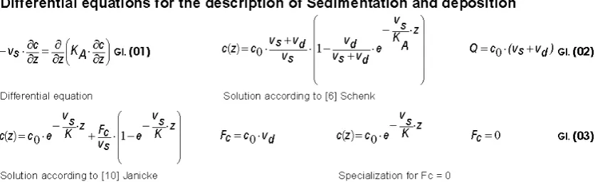
Not Only AUSTAL2000 is Not Validated
Rainer Schenk
1,21
Faculty Engineering and Environmental Sciences, Dresden University of Technology IHI Zittau, Germany 2
Department of Fluid Mechanics, Faculty of Power Plant Engineering and Energy Economics, University of Technology Zittau,Germany
Copyright©2018 by authors, all rights reserved. Authors agree that this article remains permanently open access under the terms of the Creative Commons Attribution License 4.0 International License
Abstract
On the basis of regulations and directives, since 2002 the particle model AUSTAL2000 has been mandatory in the Federal Republic of Germany for the calculation of the spread of air pollutants. In order to achieve harmonization, other model developments require that the physical basis of the AUSTAL be adopted. However, the author of this paper has variously proved that this dispersion model itself is not verified and therefore not suitable for carrying out propagation calculations. All reference solutions are faulty. Doubtful comparisons and test bills are carried out. So z. For example, 3D wind fields are compared with the rigid rotation of a solid and the position of sources is given in 200m, but their effects cannot be seen in the calculated concentration distributions. The authors of the AUSTAL address these objections with chimerical arguments and questionable definitions of deposition velocities and other dubious calculations of sedimentation and deposition currents. With each attempt to explain deepen the incomprehensibility, and you become entangled in other contradictions. This article describes that deposition currents are to be determined according to physically established laws and cannot be set arbitrarily according to amount and direction. It is shown that soil concentrations are calculated speculatively by the authors of AUSTAL. The definition of the deposition rate is substantiated physically. The author also analyzes by way of example that even further model developments are validated by the faulty reference solutions of the AUSTAL. Not only AUSTAL is not validated. In summary, further contradictions are described. AUSTAL is a further development of the dispersion model for air pollutants LASAT from the year 1984. LASAT is raised by the authors themselves and described as the mother model of pollutant spreading in Germany. For 34 years, faulty model developments have been extensively promoted.Keywords
AUSTAL2000, Sedimentation, Deposition, Deposition Rate, Dispersion of Air Pollutants1. Introduction
Within the framework of the Technical Instructions on Air Pollution Prevention according to [1] TA Luft, since 2002 the particle model AUSTAL2000 in the Federal Republic of Germany has been prescribed as mandatory for the calculation of the spread of air pollutants. To prove its suitability, other model developments must be verified with AUSTAL, which is why u.a. Reference solutions are provided. However, [2] Schenk and [3] Schenk show that all sedimentation and deposition reference solutions are flawed and that all the homogeneity tests described are only useless trivial cases. AUSTAL itself could not have been validated. The law of mass conservation and the II law of thermodynamics are violated. Further contradictions, which are to be justified with the violation of these conservation laws and main clauses, are pointed out.
In [4] Trukenmuller et al. and [5] Trukenmüller disagree
and claim that all the objections raised are due to misunderstandings and physically different ways of looking at things. Also, one would like to prove that there is an equivalence between the different specified reference solutions, what u.a. with questionable definitions of the deposition rate. All contradictions would be clarified. However, one does not know that the deposition rate is a material constant and cannot be falsified arbitrarily. However, an obvious contradiction is overlooked in all these explanations. Once one wants to counter all concerns about AUSTAL with physical evidence, but on the other hand one intends to bring about an equivalency to the correct solutions. This contradiction explains why all the efforts of the authors of the AUSTAL to refute the complaints raised in relation to their propagation model are reversed.
use the faulty reference solutions. It has also been shown that the equivalence between the two reference solutions allegedly existed by the authors of the AUSTAL cannot exist. The alleged equality is based on a deceptive derivation. Mathematics and mechanics prove that all tasks assuming a "volume source over the entire computing area" are identical and have only one trivial solution and cannot be different. Claiming that sources have been included in 200m will mislead the public. Not a single concentration profile reported by the authors of the AUSTAL suggests the presence of such sources. By means of a root cause analysis, it is clarified that the faulty reference solutions are based on an already in 1984 by [7] Axenfeld et al. can be attributed to a questionable description of all sedimentation and deposition processes. This development is dignified by the authors of the AUSTAL as the mother model of AUSTAL called LASAT.
In [8] Trukenmüller one gets involved in further
contradictions. With regard to the deposition one introduces, in addition to the already existing definitions, an additional interpretation. There is now a so-called "true deposition rate", but it is still not recognized that this can only be a material constant. The validity of BERLJAND's relation
d 0
K c / z v c⋅∂ ∂ − ⋅ =0
is denied, although it would have been recognized that it was used to derive the correct reference solution to which one wanted to bring about equivalence. Why do you even try to prove equivalence in the reference solutions, and at other times you deny the physical basics used for this. In addition, it has still not been recognized that all test cases with "volume sources over the entire computing area" distributed are equivalent trivial tasks. They relate to tasks which are identical to the simple filling of any containers with any fluids. In each considered volume of the computational domain of, for example, one cubic meter, the same emission
3
q [ g/(m s)]µ ⋅ is released, which is why at each time point t [s]
E the concentration in this container is constant and dependent only on the filling time, as can be easily understood with c t
( )
q t 0,139 3600 500 g / m3E
E = ⋅ = ⋅ = µ can
recalculate. A propagation calculation is thus completely unimportant. Already during the filling one pays attention to the fact that in each volume of the computing area the same emission is set free, and thus the concentrations are spatially constant. It is also denied that the soil sources are calculated speculatively.
In this article, using the example of case 22a with alleged sedimentation without deposition, in a single case by means of e.g. of the GAUSS integral theorem proves that the law of mass conservation and the II law of thermodynamics are violated and because of an indeterminacy in the calculation equation the soil concentrations have to be determined speculatively. The integral equation used for this purpose is concealed from the public by the authors of the AUSTAL. This article also provides proof that the BERLJAND relationship
d 0
K c / z v c⋅∂ ∂ − ⋅ =0 is physically justified. The same
argument is used to define the deposition rate.
In many cases, the author of this amount also complained that the erroneous theory for sedimentation and deposition, founded in 1984 according to [7] Axenfeld
et al. after 2002 with elaborate funding by [4]
Trukenmüller et al. developed a parallel doctrine. The
fundamentals of these different doctrines are described in the parent model of AUSTAL LASAT. Already so the dust precipitation was calculated incorrectly. This development is mainly due to the fact that all new model developments are required to be validated against the faulty reference solutions. The fact that various engineering firms also follow this call and verify their model developments on the reference solutions derived from JANICKE & JANICKE is also documented in this article. Not only the propagation model AUSTAL is not validated.
All illustrations refer to the test cases 22a, 22b, 11, 13 and 14 described in [9] Janicke) and [10]Janicke.
2. Methods and Material
Mathematics and mechanics are used alone as valid methods of incorruptible evidence to conduct subsequent investigations. By means of differential and integral equations, such as The GAUSS integral theorem for the transformation of volume into surface integrals proves that the conservation of mass and the II law of thermodynamics is violated. As further methods fluidic and thermodynamic doctrines are used to the conservation laws of momentum, heat and mass transport. In addition there are foundations of the theory of heat and mass transfer.
As material the publications of [7] Axenfeld et al., [11] Janicke et al., [9] Janicke, [12] Janicke, [13] Janicke., [4] Trukenmuller et al., [5] Trukenmüller and [8] Trukenmüller. The results of these publications are checked for correctness and plausibility using the specified methods and procedures. Further research results which are used concern the works [14] Stefanek, [15] Stefanek et a.l, [16] Schul and [17] Kubica.
3. Results
3.1. Deposition Streams are Directed against the Positive Concentration Gradient and Cannot be Determined Arbitrarily by Amount and Right
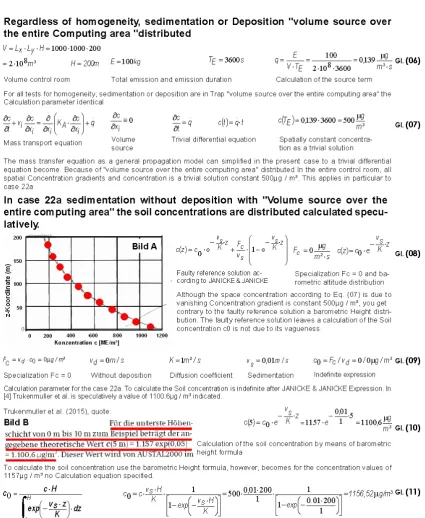
Figure 1 shows the results of the investigations carried out on the validity of the law of conservation of mass and the II. Law of Thermodynamics using the example of case 22a, sedimentation without deposition.
according to [6] Schenk and the faulty reference solution according to [9] Janicke. Equation (02) results as a correct solution of the differential equation (01). The concentration
distribution is a function of the sedimentation and deposition rate as well as of the diffusion parameter and the altitude coordinate.
[image:3.595.87.509.150.278.2]The deposition rate is an informal component of the solution. In the derivation of equation (03), the deposition rate is initially absent, which is why, without justification, the valid sedimentation stream Fc=vs⋅c0 is replaced by the deposition stream Fc =vd⋅c0 so that the deposition rate in the solution can even be used. It does not become part of the solution by taking into account the valid BERLJAND boundary condition
d 0
K c / z v c⋅∂ ∂ − ⋅ =0
, but only by arbitrariness of the authors of the AUSTAL, as can be read in [6] Schenk. The graph of Figure 1 describes the concentration curve after the faulty solution (03). The concentration gradient on the ground is negative, so contrary to all expectations for the spread of air pollutants, a deposition current of 2
11, 57 g/(mµ ⋅s) in the direction of the free atmosphere should result. The contradiction to the II. Law of Thermodynamics is that in the direction of the free atmosphere according to the solution given, a concentration compensation by conduction should take place, but it is stated that it disappears due to lack of deposition with vd=0 m/s , but what the adjacent
concentration gradient contradicts. The specified concentration curve forces an equipotential bonding in the direction of the free atmosphere and cannot be chosen freely in terms of magnitude and direction. Not only by these considerations, the calculated concentration course is doubtful. The given concentration distribution could only be understood if one laid the source in the ground, which in addition to all the absurdity but also the assumption "volume source over the entire area of the law" distributed again would contradict. These relationships are described by equations (04). By applying the GAUSS integral theorem, equations (05) explain that solution Eq. (03) with the "specialization Fc = 0" violates the mass conservation law.
All inconsistencies, which are revealed as a consequence of the faulty reference solutions, could thus be elucidated using the example of case 22a.
3.2. For Sedimentation and Deposition, the Soil Concentrations are Calculated Speculatively
Before all the peculiarities of the case 22a, can be further discussed, it should be remembered that according to [9]
Janicke and [10] Janicke, all verification tests are divided
into two groups. On the one hand, it is homogeneity tests and, on the other hand, it is tests for sedimentation and deposition. Finally, case 21, deposition without sedimentation, case 22a, sedimentation without deposition, and case 22b deposition with sedimentation are described. By Fc=vd⋅c0 we mean "the mass flow density forced by the source" or, in the case 22b, a "source strength of
2 c
F = µ1 g/(m s)⋅ ". Accordingly, Fc is the release of
emissions. Depending on the case example, a specialization is used for Fc.
Now, with a known deposition rate
v
d and given swelling strengthc
F with the relation Fc=vd⋅c0 , it is possible to determine the soil concentration c0=F / vc d, as
was also the case in cases 21 and 22b. There, the soil concentrations amount to 3
0
c =15 g/mµ and c0=20 g/mµ 3. In both these cases, it is possible to proceed in such a way that the deposition velocity is different from zero, vd ≠0 . The emissions amount to Fc= µ1 g/(m2⋅s) and should have been located at 200m, which could not have been, according to [6] Schenk. Depending on how the source strength
c
F
is determined, without having to use an analytical solution, the soil concentration is already obtained, which is very surprising, at least for the case 22b.With regard to the calculation of the soil concentration , however, the situation is different in case 22a. Here no deposition should take place, which is why the deposition rate must be assumed to be vd =0 m/s. This results in the used "specialization Fc= µ0 g/(m2⋅s)" for this case. It is now the case that no equation of determination is available for the calculation of the soil concentration. This results in an indefinite expression 3
0
c =0 / 0 g/mµ . This expression makes it possible to arbitrarily set or somehow determine the soil concentration. The appropriate solution function, which one would have had to develop from the relevant differential equation (1), is not suitable because of its erroneous derivation and indeterminacy. It will be of interest how the authors of the AUSTAL proceed. Because of the
c
"Spezialisierung F=0", the erroneous reference solution c z( ) c exp v z/k0 s F / v 1 exp v z/k c s s
= ⋅ − ⋅ + ⋅ − − ⋅
reduces to a simplified exponential function
( ) 0 s
c z c exp v z/k
= ⋅ − ⋅ in which the soil concentration is the only unknown. To calculate the soil concentration, a further determination equation has to be developed. The simplest case of a disappearing soil concentration
3 0
c = µ0 g/m is excluded, because otherwise the whole problem of the case 22a would be in question. A solution function based on the differential equation (1) is likewise not available because of the described vagueness, which is why it is necessary to help one another.
In this predicament speculate the authors of the AUSTAL and use the case 11 of the homogeneity test. There, as in all other cases, the same geometrical relations exist for homogeneity, and there already at a total emission of E=100 kg and a filling time of TE=3600 s a constant
concentration of space c=500 g/mµ 3=konst. was found to be the solution of the trivial Differential equation determined. However, it was assumed that a "volume source over the entire computing area" was distributed at
3
q=0,139 g/(mµ ⋅s) and not from an area source in the
0
dimension µg/(m2⋅s) . One ignores this difference and now transfers this source type to case 22a as well, although in all other tests of this group one assumed a surface source of Fc=vd⋅c0 . For the present case 22a, the
c
"Spezialisierung F 0"= would have meant that no emissions could have occurred in the entire control room, which would have been understandable with a vanishing soil concentration of c0= µ0 g/m3 . But because this triviality is contrary to the whole task, one has to rely on a different explanation about the origin of emissions. For this reason, the authors of the AUSTAL use the source form of case 11 "volume source over the entire computing area" distributed. Obviously, the source types are changed arbitrarily by the authors of the AUSTAL as needed. However, in the case of this substitution, one overlooks the fact that the same problem exists for case 22a because of the spatial concentration gradients that vanish here, as in case 11, and that a solution deviating from
3
c=500 g/mµ =konst. cannot exist at all, as in [6] Schenk
was detected. This fact is ignored. As the authors of the AUSTAL now proceed, with means of mathematics and mechanics is no longer explainable. They compulsorily distribute the mass of E=100 kg in the control room of case 11 so that the new distribution satisfies its erroneous exponential function c z( ) c exp v z/k 0 s
= ⋅ − ⋅ . From this
consideration, the [4] Trukenmüller et al. cited soil concentration of c0=1156,52 g/mµ 3. However, the reader does not learn how this concentration value is calculated. A calculation equation is not specified. It turns out that the authors of the AUSTAL conceal the relationship used for
this v Hs
c c v H / K 1/ 1 exps
0 K
⋅
= ⋅ ⋅ ⋅ − − . However, knowing this
equation would be necessary if other authors of model developments want to validate their algorithms. This approach is speculative and not physically substantiated. If
one compares this with comparisons of procedural mixing, this redistribution would be equivalent to demixing, but this would be understandable only with an energy input, which, however, can not be mentioned here.
The conditions can be easily understood using the example of Figure 2. Equations (6) describe the geometrical relationships of cases 11, 13, 14 and 22a. In all cases, it is assumed that there is a "volume source over the entire computing area". The specific source term is
3
q=0,139 g/(mµ ⋅s) t. The equations (7) explain that all spatial concentration gradients must disappear due to this volume source. The concentration adjustment of
3
c=500 g/mµ =konst. has occurred after the end of the emission after TE=3600 s and not after 10 days, as
claimed by the authors of the AUSTAL. According to Eq. (08) and Fig. A, the simplified exponential function for the concentration distribution is given by
c
"Spezialisierung F=0", in which the soil concentration still has to be determined. That one receives an indefinite expression for this, describe the equations (09).
In [4] Trukenmuller et al. we want to explain, according to
picture B, how the soil concentration is calculated. For this one needs the concentration value in the amount of
3
1157 g/mµ , for which however no calculation equation is specified. According to equation (10), the concentration of
( )
3c 5 =1100,6 g/mµ at a height of 5 m is determined and used as the valid soil concentration below. Equation (11) describes the secretive equation for the determination of the required concentration value of 1157 g/mµ 3, without which validation of propagation models is not possible. None of the publications and program descriptions issued to AUSTAL mention how to calculate this value. This also applies to the relevant VDI regulation [18] VDI 3945 Part 3.
0
Figure 2. Speculative calculation of soil concentration
The authors of the AUSTAL calculate the soil concentration speculatively and mislead all model developers and the public.
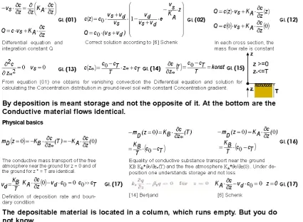
3.3. Deposition Rate and Calculation of Deposition Currents
As mentioned in the introduction, [7] Axenfeld et al. in 1984 developed a model for the calculation of dust
precipitation. This mother model LASAT was developed in 2002 to AUSTAL2000. There, according to SA (01), the deposition rate
v
d is defined as the velocity with the"-picturally speaking -... a pillar standing up on the earth's surface, which contains the material capable of being
deposited," runs empty by deposition " („-bildlich
gesprochen-... eine auf der Erdoberfläche aufstehende Säule, welche das depositionsfähige Material enthält,
and in [8] Trukenmüller it is supplemented and claimed that one could use the equation or
as the definition equation for the deposition velocity. Both verbal and mathematical formulation is incomprehensible and contradictory. The result is the need to show these opposites and bring about a clarification.
First, the model concept, which underlies the relevant differential equation (01), will be explained. This states that a constant stationary flow of air admixtures moves convectively and conductively vertically downwards. The convective material flow is formed by the product of flow velocity and concentration , and the conductive material flow results from the product of diffusion coefficient and concentration gradient . With a positive gradient, it is directed counter to the positive z-coordinate. The sum of the individual partial flows is constant vertically upwards in each cross section of the control room. While the sediment
v
s⋅
c
0 deposits on the ground, the conductive streamv
d⋅
c
0 is deposited in the soil. Storage is understood to mean storage and not the opposite of loss. To comply with stationary observation, the sediment must be mechanically removed continuously, e.g. in the case of surface winds and other whirling up. In the example of a procedural exhaust gas purification is comparatively a discontinuous cleaning of filter surfaces. The deposition stream penetrates into the interior of the soil and leads to an enrichment of the soil with the pollutant in question. The model assumes that the soil has an unlimited capacity, which cannot be avoided in a stationary observation. Examples include the penetration of aerosols into the soil or its acidification by sulfur-containing air admixtures. Other examples include the penetration of radionuclides into the subsurface and the consequent enrichment with radioactive decay products. Assuming a limited absorptive capacity of the soil, a transient approach is imperative. In this case, a complete equipotential bonding in the free atmosphere and in the soil will lead to a constant concentration distribution throughout. The compensation time results as a solution of an initial boundary value task, however, the model equation (01) has to be extended by the temporal change of the concentration and by the source term q µg / (m3⋅s , Eq. (07). Due to the lack of convection in the ground, the propagation is described by the differential equation.
The conditions are explained further in Figure 3. The equations (01) describe for a stationary consideration the differential equation with the still unknown integration constant Q , which results after a single integration. Subsequent application of the "LAGRANGE method" results in the solution (02) and the integration constant Q
as the sum of the convective and conductive mass flows. The analytic relationship Q c (v v )
s
0 d
= ⋅ + belongs to the
differential equation and cannot be arbitrarily exchanged
for the deposition current vd ⋅c0 , as the authors of the AUSTAL in [4] Trukenmüller et al. and [8]
Trukenmüller. The boundary condition is a constant soil
concentration and a constant mass transfer between ground-level atmosphere and soil. The constancy of the mass flows explains the equations (12), and the penetration of the pollutant into the soil near the ground is described by the differential equation (13). It is identical to the differential equation (01), but there is no convective flow in the soil, vs=0. As a solution, equations (14) and (15) show a linear concentration distribution in the soil, and thus a constant concentration gradient everywhere
( )
c / z z∗ ∗ konst.
∂ ∂ = . The equality of the conductive mass flows as a boundary condition is described by Equations (16) using the constant concentration gradient of Equation (15). Assuming that the concentration cT at ground depth is negligible with respect to the soil concentration ,
c c
T
0>> , we obtain the equation (17), which arises from the requirement of equality of the conductive mass flows at the Bottom limit results. At the same time, the definition of the deposition rate is obtained as the quotient between the effective mass transport coefficient in the soil and a measure of length which characterizes an indefinite soil depth, vd=K / T m/sB . This definition also justifies that the deposition rate is a material constant. The parameters
B
K und T depend on the soil conditions on the surface and on the interior of the soil. The deposition rate thus formed is usually determined experimentally. The deposition rate does not result from a parameterization. It is physically based on the equality of the conductive material flows on the ground. The boundary condition is identical to the relationship given in [19] Berljand, Eq. (17). The deposition rate is equivalent to the mass transfer coefficient
m/s
β . The correctness of the calculation is confirmed by combining equation (12) for z=0 with the integration constant . The boundary condition (17) is also substantiated and successfully applied in [14] Stefanek.
As is well known, the product of speed and mass density leads to mass flow. In the case that the velocity is the deposition rate, the result describes a deposition current. If, however, it is a sedimentation rate, this results in a sedimentation stream. The sum of both explains the total mass flow. However, one cannot say the deposition rate and at the same time claim that the result would be the total mass flow, as stated in [8] Trukenmüller. Although it is possible to parameterize a deposition rate as desired, integration constants are not determined from parameterized boundary conditions but from physically justified boundary conditions.
In contrast to this approach, the authors of the AUSTAL lack the second boundary condition as a consequence of a mass constancy at the boundary surface of the Earth's
d v c c
F = 0⋅ vd=Fc/c0
( )
z c s v ⋅( )z z / c A K ⋅∂ ∂
−
[
g/(m³ s]
t /
c ∂ µ ⋅
∂
(
KB c/z)
bzw. 0 c/(
z z)
z / t /
c ∂ =∂ ∂∗ ∂ ∂ ∗ =∂2 ∂ ∗∂ ∗
∂
d v c c F = 0⋅
surface. Equation (12) is related to the relationship used by the authors of AUSTAL
in [4] Trukenmüller et al., identical, only for the
integration constant Q and the diffusion coefficient K modified formula symbols are used. In this respect, the considerations can be continued with the identities (23) shown in Figure 3. The authors of the AUSTAL thus use the equation (12). Instead of determining the resulting integration constant by means of the LAGRANGE method, this is unfounded replaced by a deposition current, which will turn out to be deceptive. Equation (12) consists of two summands, the first of which describes the sedimentation stream c
( )
0 ⋅vs and the second KA⋅∂c/∂z( )0the conductive substance stream. The authors of the AUSTAL misunderstand that the second summand with
( )
A
K c / z 0 0 d
c v
⋅ ≡
⋅ ∂ ∂ according to Eq. (17) is identical tothe deposition current at the bottom, and thus
( )
0( )
0 00⋅vd=c ⋅vs+c ⋅vd⋅→ vs=
c shows that no
sedimentation current should occur, equations (18). The integration constant Q is replaced by , Eq. (19). This conclusion, however, contradicts the original task according to differential equation (01), where one would like to take into account a sedimentation stream. Thus, the equation (19) is erroneously obtained, which according to the relation (20) is actually an inequality. So is the equation (21) after [7] Axenfeld et al., which is described below with Eq. (22) was incorporated into the Handbook Urban Climate as a scientific handbook for practice in environmental planning in 1988, which can be read in [20] VDI Commission Clean Air. The erroneous equation (19) is at the same time regarded as a boundary condition, although its development is not based on any physical considerations. The parent model LASAT also
uses this self-conceived boundary condition. It results solely from incorrectly used mathematical formalities. The inaccurate relationship is used in [4]
Trukenmüller et al. derived the erroneous reference
solution (02) from the authors of the AUSTAL. As will be shown below, other authors of model developments subsequently validate their algorithms on this incorrect reference solution, which implies that not only AUSTAL is not validated. Also all other developments, which use the complaint model bases of the AUSTAL, are not validated. Due to a lack of reasoning based on physics, one cannot give a conclusive definition of the deposition rate and loses itself in questionable formulations. These statements also apply to the parent model LASAT. As already mentioned, according to theorem SA (01), a pillar standing up on the earth's surface should run empty. However, it does not explain how the depositable material could get into this column and where it is when it has run empty. This thought construction proves the incomprehension of the authors of the AUSTAL, with which one would like to describe sedimentation and deposition processes.
Another contradiction is to be pointed out. In [4]
Trukenmuller et al. we want to justify the validity of the
reference solution (03) and in [8] Trukenmüller the usability of the faulty boundary condition according to equations (19) and give a definition of the deposition rate. In both cases, the integration constant Q is replaced by the deposition current to . In the first case, this obscures the appearance of a trivial solution c=konst.
because the actual sedimentation stream
( )
z vi c( )
z vs cc
F = ⋅ = ⋅ is replaced by a deposition stream
c d v c
F = ⋅ 0 .
( )
z vs c( )
z z/ c K c
F = ⋅∂ ∂ + ⋅
Q
d v c p F c
F = = 0⋅
d v c p F c
F = = 0⋅
d v c p F c
Figure 3. Parametrized and physically justified deposition rates
This castling is physically unfounded and arbitrary, resulting in a violation of mass conservation. How to do this is explained in detail in [6] Schenk. In the second case, one does the same thing, but fails to recognize that it provides another trivial solution. It turns out that because of
( )
00 vd KA c/ z
c ⋅ ≡ ⋅∂ ∂ no sedimentation velocity can occur,
In conclusion, it should be noted that equation (01) is an ordinary differential equation of the second order. According to the theory of ordinary differential equations, two integration constants arise in the solution process. Both are to be determined by means of physically justified boundary conditions. If physics is indisputable, there are also undisputed solutions. In the present case, one has a boundary condition with c
(
z=0)
=c0, but the authors of the AUSTAL lack a further physically justified rule with which one could determine the second integration constant. One resorts to controversial definitions of the deposition rate and entrenches itself subsequently engrossed in contradictions. With these statements it was shown that the disastrous development of the AUSTAL had already begun in 1984 with the LASAT model. The causes for this were physically justified.It can be assumed that the differences formulated above for the definition of the deposition rate and for the calculation of deposition currents can be regarded as sufficiently clear.
3.4. Validation on Analytical Solutions and Reference Examples
High demands are placed on the development of algorithms for the solution of differential equations of mathematical physics. First, it must be made clear that physically justified model equations are available. The field of fluid mechanics is determined by experimental and theoretical studies on the movement of liquids and gases. Fluids and gases almost one together under the collective term fluids. A distinction is made between compressible and incompressible fluids. The movement of these fluids is described by the NAVIER-STOKES differential equations. They are the basic equations of fluid mechanics. If the fluids are used as carrier media for heat and material, then further balance equations are added. One then speaks of the coupled differential equation system of momentum, heat and mass transport, which finds application in many scientific disciplines adjacent to fluid mechanics. The spread of air bubbles takes place in the PRANDTL layer, which is why fluid mechanics and thermodynamics are primarily concerned with the motion processes in this layer. Because air pollutants are basically transported in a carrier medium, one speaks of a mass transfer equation. When heat is moved so, this is accounted for by the heat transfer equation. In this way, pulse is moved by the NAVIER-STOOKES differential equations. The coupled differential equation system thus described thus accounts for the transport quantities momentum, heat and material. All these transport processes have an analogy in common. It consists in that these transport sizes are moved equally by convection and conduction. They are in a carrier medium, e.g. Air, stored and continue with the flow. This form of moving is called convective transport. Conductive transport describes the balance of momentum, heat and matter through the occurrence of friction, conduction and
diffusion.
functions and GAUSS distributions for the propagation of air pollutants, the flow near oscillating walls as well as the flow between rotating cylinders. Other other examples are described extensively in [21] Schlichting, [22]
Truckenbrodt, [19] Berljand, [23] Albring and [24] Naue.
In order to study the effect of the Coriolis force, the
EKMAN spiral
( )
(
)
(
)
g
u z= ⋅ −u 1 exp z/D cos z/D − ⋅ and
( )
exp( z / D) sin z / D( )g
v z
= ⋅
u
− ⋅ are often used inmeteorology. This integral of the equations of motion is also available. Useful numerical methods are shown and explained, for example, in [25] Yanenko. For example, methodological foundations and practical applications for the validation of propagation models are described in detail
in [17] Kubica and [16] Schul. A stable and consistent
method for the numerical solution of transport equations explains [15] Stefaneket al. As far as flow and dispersion models are concerned, a distinction is made between diagnostic and prognostic procedures. While the diagnostic models examine existing flow and propagation situations, predictive models can predict future solutions. Flow and dispersion models are developed as part of university and non-university research. The university-developed models have the advantage that they are usually completed with academic graduations, and quality assurance is ensured.
As regards the propagation model AUSTAL, one would like to validate it as well. However, it should first be noted that the reader does not learn which model equation of the development is the basis. Neither in [13] Janicke et al. still
in [10] Janicke is written about it. Only in [9] Janicke it is
pointed out that in [19] Berljand the general mass transfer equation, which is sometimes called the diffusion equation, is used, but not by the authors of the AUSTAL itself. Reference is made in this connection to the VDI Guideline
[18] VDI 3945, but one cannot find out there about a
propagation model used. It is therefore not clear how the already erroneously formulated homogeneous and inhomogeneous turbulence approaches are used. For example, one does not know whether it is stationary or transient model considerations. In the solution method one
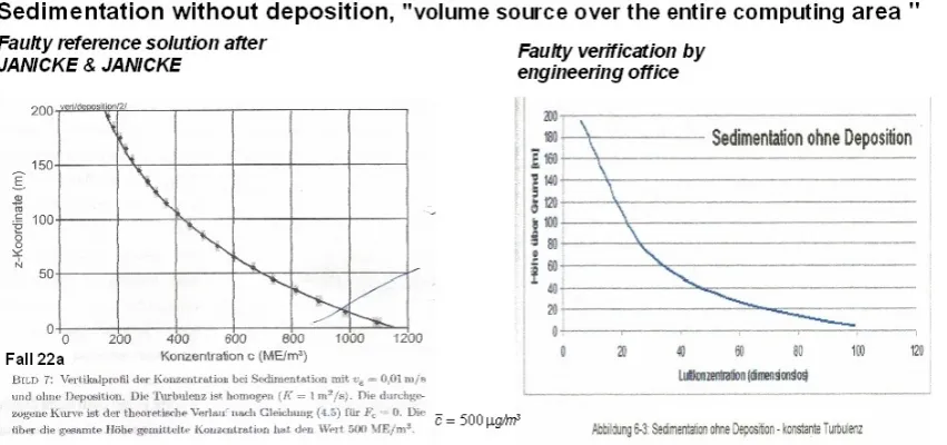
explains the choice of constant as well as not constant time steps and points to compensation times of 10 days, after which the stationary state should have set for all calculation examples. Therefore, one has to believe that transient calculations are performed, but no single time-dependent analytic solution is given to validate this transient behavior. Therefore, it cannot be said that one can count time series. Reference has already been made to the importance of stable numerical methods. The authors of the AUSTAL themselves write that solutions cannot converge. This information raises legitimate doubts about physics, which AUSTAL uses to model propagation processes. It is due to the nature of unstable numerical methods that these divergences can only occur for a short time. However, after any instability that has occurred, the calculation will continue with an error that has occurred. It comes to a fault continuation, where in the end it is difficult to judge what you have received for a solution. The sedimentation and deposition reference solutions given by the authors of the AUSTAL and all homogeneity tests are flawed and not suitable for validation. It is deceptively claimed that the solution was validated on 3D wind fields. In fact, one uses the rigid rotation of a solid. The authors of the AUSTAL lack the idea that one could at least use the EKMAN spiral known in meteorology. By forming integral averages, e.g. with the BERLJAND profiles, faulty solutions are smoothed out. Nevertheless, the error deviations are still up to 70%, which increase even further with a reduction in the source distance. Bessel functions are calculated incorrectly. It is reported by users that AUSTAL also calculates concentrations within closed borders. One explains this incomprehensibility with the fact that particles cannot see house walls, but want through. Such phenomena are more indicative of programming errors than equipping pollutant particles with vision. These and other differences, as described for example in [2] Schenk and [6] Schenk, prove that AUSTAL could not be validated.
Figure 4. Validation for the reference cases sedimentation with and without deposition
AUSTAL was released in 2002. The intention was to achieve a harmonization of all propagation calculations, which means that all further model developments have to use the same model fundamentals. For this reason, [18]
VDI 3945 publishes reference solutions and other
procedural principles, and requires all model developers to validate their algorithms against these dubious foundations and erroneous reference solutions. But as already described, all reference solutions and homogeneity tests are flawed.
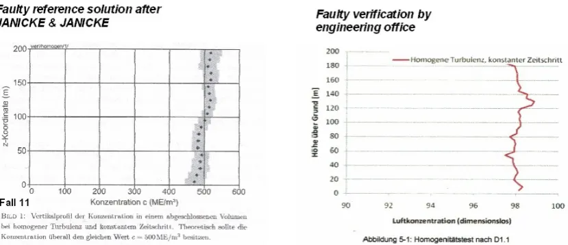
The situation is now to be assessed in such a way that most model developers understandably rely on the published rules for validation and verify their algorithms. They respect the authority of the clients of the AUSTAL and rely on credibility. In any case, model developers prove that their algorithms are equivalent to those of the AUSTAL, as shown in Figures 4 and 5, for example.
for the individual case examples, and on the right, according to [27] N.N., for example, shows the corresponding graphics of an engineering office. As can be seen, the AUSTAL solutions show a satisfactory agreement, which proves that this model development is also flawed and not suitable for carrying out dispersion calculations. While Figure 4 describes all tests for sedimentation and deposition, Figure 5 is all homogeneity tests.
The above statements show that other propagation models have also been validated against the erroneous reference solutions of the AUSTAL. Not only AUSTAL is not validated.
[image:13.595.91.506.246.425.2]The authors of [4] Trukenmüller et al. provide information. However, there are also propagation models of engineering firms which meet all requirements, but must subsequently validate themselves against the faulty reference solutions of the authors of the AUSTAL. How to do this is easy to recognize.
4. Discussion
The results of this article and other contradictions of the propagation model AUSTAL can be discussed in summary.
In the case of the reference trap 22a of the AUSTAL, it was demonstrated that the specified solution course is faulty. There should be no deposition, but the course of concentration suggests that a conductive material flow should be directed against all conditions in the free atmosphere. By means of integral theorems it has been proved that the II law and the mass conservation law are violated.
For the calculation of the soil concentration for the case 22a, an indeterminate expression results due to the erroneous reference solutions. A calculation equation is not available. For this reason, a "volume source over the entire computing area" is selected for this case alone as for all homogeneity tests. This gives you the opportunity to calculate the soil concentration speculatively. A formerly constant concentration distribution is converted in such a way that the concentration distribution follows the erroneous barometric height distribution given by the authors of the AUSTAL. The calculation equation for this is concealed from the public because of its obvious lack of credibility. It is specified by the author of this article and all associated incomprehensibilities are cleared up. The authors of the AUSTAL are obviously trying to mislead the public with their model development.
Depositing is storage and not loss. The depositable material penetrates into the soil and is distributed there. This results in a conclusive definition of the deposition rate. The integration constants of differential equations are not determined from parameterized rules, but, in contrast to [8]
Trukenmüller, by means of physically justified boundary
conditions.
Guidelines and regulations require all model designers to validate their propagation algorithms against the erroneous reference solutions of the authors of the AUSTAL. By way of example, it is shown that this request was also followed. Not only AUSTAL is not validated. [4]
Trukenmuller et al. can provide information on further
such model developments.
Eight reports are available for the evaluation and evaluation of AUSTAL. The authoritative statements of the authors of the AUSTAL are not very manageable. The reader has to painstakingly collect the physical and mathematical basics individually.
All reference solutions for homogeneity, sedimentation and deposition are faulty.
By means of integral sentences, such as The GAUSS integral theorem proves that the violation of the Second Theorem of Thermodynamics and the Law of Mass Conservation is not limited to individual cases. The general validity of the objections raised has been proven.
One tries to bring about an equivalency between the
erroneous and correct reference solutions. For this one introduces deceptively different definitions of the deposition rate, but fails to recognize that this is a material constant, which cannot be defined arbitrarily.
In 1984 LASAT was developed for the calculation of dust precipitation. LASAT is referred to by the authors of the AUSTAL as the mother model of pollutant propagation. In the context of a root cause analysis it could be proven that physically unfounded ideas of deposition and sedimentation lead to faulty boundary conditions. The material capable of being deposited should stay in a column, which henceforth runs empty. But you cannot explain where the material should be after that. This erroneous model presentation is adopted as a novel doctrine in a scientific handbook on environmental planning. Also, the algorithm of the parent model LASAT calculates incorrectly.
All cases of homogeneity, sedimentation and deposition use a "volume source over the entire computing area" distributed. The authors of the AUSTAL misjudge that the resulting task equals the filling of a container. The emission duration of one hour is identical to the filling and equalizing time. With the end of the issue, a complete concentration equalization has already taken place and not just after 10 days, as the authors of the AUSTAL state.
Because of the "volume source over the entire computing area" distributed, disappear at the beginning of the filling all concentration gradients. Thus, all homogeneity tests and the case 22a describe the same tasks, but for each individual case different solutions are given. How to validate propagation models is inexplicable.
Sources are said to have been located at 200m, but there is no single course of concentration that would reveal the effect of high altitude sources. The authors of the AUSTAL speculate on ignorance.
In addition to the homogeneity, sedimentation and deposition tests, AUSTAL also wants to validate on a 3D wind field. Instead of using such a velocity distribution, one uses the rigid rotation of a solid in the plane. The possibility of validating their model on at least the well-known EKMAN spiral misses the authors of the AUSTAL as well. Again, one relies on ignorance.
BERLJAND profiles describe three-dimensional concentration distributions. They claim to have compared their own simulation results with it. However, instead of using these profiles, only two-dimensional integral means are compared. Numerical errors are smoothed and hidden. Nevertheless, the deviation in the near range is still more than 70%. The position of the concentration maximum away from the source point is calculated with an error of approx. 30%. The calculation of safety distances is affected.
consistency. In all reports of the authors of the AUSTAL this is nothing to experience.
Homogenizing is confused with diffusion. Homogenization, like crushing, is one of the basic operations of process engineering. While an energy input is responsible for the mass balance during homogenization, in the case of diffusion, the mass transfer occurs in the opposite direction to the concentration gradient. In the case of diffusion, a potential gradient is responsible for the concentration balance.
One pretends to be able to calculate time series, but no single analytical solution is given, with which AUSTAL could have validated also on transient solutions.
The authors of the AUSTAL state that particles cannot see house walls, yet they want to go through them. Obvious programming errors should be obfuscated. Numerical algorithms can be developed without errors by using modular programming. Teaching examples can be found in
[14] Stefanek, [15] Stefanek etal. and [26] Schul read.
As can be seen from the non-university research on the example of the modeling of the spread of air pollutants, one can learn In [28] UBA: “The history of AUSTAL2000 started almost exactly 21 years ago. At the NATO CCMS conference in San Francisco, which took place end of August 1981, I had just presented my formulation of Lagrangian modelling in inhomogeneous turbulence, parallel to similar works by Wilson and Legg & Raupach; in doing so, I delivered a promise made to Hanna during a conference in the preceding year in Amsterdam. The preparations for the TA Luft 1983 had not yet finished,
nevertheless the participants already discussed how the TA Luft should develop on an intermediate and long-term time scale. After the conference, we therefore sat together in the small village Kirkwood, in the mountains east from Jackson, in order to bring our ideas together (in the framework of the UBA project "handbook for immission calculations"). We, that was: Werner Klug, Paul Lühring, Rainer Stern, Robert Yamartino, and myself. Key points for a long-term concept that should reach about 5 to 7 years into the future were, among others: Now, after 21 years, major points of that former concept have been realised with the new TA Luft that came into force at October 1, 2002. Maybe one should meet again in the mountains and discuss how the dispersion model of the TA Luft should develop over the next 20 years….Lutz Janicke, 30.09.2002”.
5. Conclusions
Mathematics and mechanics proved that AUSTAL was developed in a chimerical way. This applies to all further model developments that have been validated on the faulty reference solutions. Not only AUSTAL is not validated. Security plans and, for example, security analyzes prepared with AUSTAL are to be reviewed. These statements are also true for the LASAT declared by the authors of the AUSTAL to the parent model. It is recommended to pay more attention to the results of university research. They guarantee a high quality.
REFERENCES
[1] TA Luft: Erste Allgemeine Verwaltungsvorschrift zum Bundesimmissionsschutzgesetz, GMBI, 2002.
[2] Schenk, R.: AUSTAL2000 ist nicht validiert, Immissionsschutz 01.15, S. 10 – 21.
[3] Schenk, R.: Replik auf den Beitrag „Erwiderung der Kritik von Schenk an AUSTAL2000 in Immissionsschutz 01/2015“, Immissionsschutz 04.15, S. 189 – 191.
[4] Trukenmüller, A.; Bächlin, W.; Bahmann, W.; Förster, A.; Hartmann, U.; Hebbinghaus, H.; Janicke, U.; Müller, W. J.; Nielinger, J.; Petrich, R.; Schmonsees, N.; Strotkötter, U.; Wohlfahrt, T.; Wurzler: Erwiderung der Kritik von Schenk an AUSTAL2000 in Immissionsschutz 01/2015, Immissionsschutz 03/2015, S. 114 – 126,
[5] Trukenmüller, A.: Äquivalenz der Referenzlösungen von Schenk und Janicke, Abhandlung Umweltbundesamt Dessau-Roßlau, 2016, S. 1 - 3, IBS Archiv.
[6] Schenk, R.: The Pollutant Spreading Model AUSTAL2000 Is Not Validated, Environment and Ecology Research 5(1), 2017, S. 45-58.
[7] Axenfeld, F.; Janicke, L.; Münch, J.: Entwicklung eines Modells zur Berechnung des Staubniederschlages, Umweltforschungsplan des Bundesministers des Innern Luftreinhaltung, Forschungsbericht 104 02 562, Dornier System GmbH Friedrichshafen, Im Auftrag des Umweltbundesamtes, 1984.
[8] Trukenmüller, A.: Stellungnahmen Umweltbundesamt vom 10.02.2017 und 23.03.2017, Dessau-Roßlau, 2017, S. 1-15, IBS Archiv.
[9] Janicke, L.: IBJparticle, eine Implementierung des Ausbreitungsmodells, Bericht IBB Janicke, 2000.
[10] Janicke: AUSTAL 2000, Programmbeschreibung, Dunum, 2002.
[11] Janicke, L.; Klug, W.; Rafailides, S.; Schatzmann, M.; Strimaidis, D.; Yamartino, R.: Validierung des „Kinematic Simulation Particle Model (KSP-Modell) für Anwendungen im Vollzug des BImSchG, Bericht 98-295 433 54 des Bundesministerium für Umwelt, Naturschutz und Reaktorsicherheit, Hamburg 2000.
[12] Janicke: Ausbreitungsmodell LASAT Referenzbuch zur Version 2.10, Dezember 2001.
[13] Janicke, U.; Janicke, L.: Entwicklung eines Modellgestützten Beurteilungssystems für den Anlagenbezogenen Immissionsschutz, IBJanicke, 2001.
[14] Stefanek, G.: Entwicklung einer Softwareapplikation zur Berechnung der Ausbreitung von Luftschadstoffen für Aufgaben auf dem Gebiet der Umwelttechnik. Technische Universität Dresden, 2002, IHI Zittau.
[15] Stefanek, G. u.a.: Eindimensionale Wärmeleitungsgleichung am Beispiel des Bodenwärmestromes. UT00, Technische Universität Dresden, MUT00, 2001, IHI Zittau.
[16] Schul, J.: Modellierung der Ausbreitung von Verkehrsschadstoffen am Beispiel der Stadt Zittau. Technische Universität Dresden, 1998, IHI Zittau.
[17] Kubica, M.: Durchführung von numerischen Experimenten zur Validierung Ausbreitungsmodells LIMA STAUB am Beispiel des Tagebaues Hambach. Technische Universität Dresden, 2007, IHI Zittau.
[18] VDI 3945, Blatt 3: Umweltmeteorologie – Atmosphärische Ausbreitungsmodelle-, Partikelmodell, Beuth Verlag Berlin September, 2000.
[19] Berljand, M., E.: Moderne Probleme der atmosphärischen Diffusion und Verschmutzung der Atmosphäre, Akademie-Verlag Berlin, 1982.
[20] VDI Kommission Reinhaltung der Luft: Stadtklima und Luftreinhaltung, Springer Verlag, 1988.
[21] Schlichting, H.: Grenzschichtheorie, Verlag G. Braun, Karslruhe, 1964.
[22] Truckenbrodt, E.: Fluidmechanik, Springer Verlag, 1989.
[23] Albring, W.: Angewandte Strömungslehre, Akademie Verlag Berlin, 1961
[24] Naue, G.: Einführung in die Strömungsmechanik, Reprocolor Leipzig, 1967.
[25] Yanenko, N. N.: Die Zwischenschrittmethode zur Lösung mehrdimensionaler Probleme der mathematischen Physik, Springer Verlag, 1969.
[26] Schul, J.: Entwicklung der Graphiksoftware IMPRES zur Visualisierung von instationären Verkehrsimmissionen. Technische Universität Dresden, 1998, IHI Zittau.
[27] N.N: Verifikation nach VDI 3945 durch Ingenieurbüro, 2009, IBS Archiv.