Tree-based Threshold Model for Non-stationary Extremes
with Application to the Air Pollution Index Data
Afif Shihabuddin
1,
Norhaslinda Ali
1,2,∗,
Mohd Bakri Adam
1,21InstituteforMathematicalResearch,UniversitiPutraMalaysia,43400UPMSerdang,Selangor,Malaysia 2DepartmentofMathematics,FacultyofScience,UniversitiPutraMalaysia,43400UPMSerdang,Selangor,Malaysia
Received July 01, 2019; Revised August 22, 2019; August 30, 2019
Copyright c2019 by authors, all rights reserved. Authors agree that this article remains permanently open access under the terms of the Creative Commons Attribution License 4.0 International License
Abstract
Air pollution index (API) is a common tool used to describe the air quality in the environment. High level of API indicates the greater level of air pollution which will gives bad impact on human health. Statistical model for high level of API is important for the purpose of forecasting the level of API so that the public can be warned. In this study, extremes of API are modelled using Generalized Pareto Distribution (GPD). Since the values of API are determined by the value of five pollutants namely sulphur dioxide, nitrogen dioxide, carbon monoxide, ozone and suspended particulate matter, data on API exhibit non-stationarity. Standard method for modelling the non-stationary extremes using GPD is by fixing the high constant threshold and incorporating the covariate model in the GPD parameters for data above the threshold to account for the non-stationarity. However, high constant threshold value might be high enough on certain covariate for GPD approximation to be a valid model for extreme values, but not on the other covariates which leads to the violation of the asymptotic basis of GPD model. New method for the threshold selection in non-stationary extremes modelling using regression tree is proposed to the API data. Regression tree is used to partition the API data into a stationary group with similar covariate condition. Then, a high threshold value can be applied within a group. Study shows that model for extremes of API using tree-based threshold gives a good fit and provides an alternative to the model based on standard method.Keywords
Air Pollution Index, Threshold Exceedances, Generalized Pareto Distribution, Non-stationary, Regression Tree, Tree-based Threshold1
Introduction
Air quality is an important aspect of human life. In Malaysia, it is monitored and enforced by the Department
of Environment (DOE). Air quality is determined by the Air Pollution Index (API) which is updated hourly by DOE. API value is derived from five main pollutants which are ground level ozone (O3), nitrogen dioxide (NO2), particulate matter
(PM10), carbon monoxide (CO) and sulphur dioxide (SO2).
High concentration of these pollutants in the air is harmful for everyone and also causing serious health problem. High concentration of SO2, NO2 and CO in the air can cause a
heart and lungs problem [1]. High level of PM10is associated
with haze days which can limit the eyesight and cause the respiratory problem [2]. According to Malaysian Ambient Air Quality Guidelines (MAAQG), API values which above 100 are considered unhealthy and could threaten public health. Therefore it is important to understand the behavior of high level of API particularly to give health warnings for the public. In order to describe the behavior of high level API at a particular area, it is important to identify the distributions which best fit the data [3]. Extreme value distribution from extreme value theory are suitable in modelling such high values.
analysis (EVA) in the context of air pollution data set in many parts of the world. An early comprehensive review of the application of EVA to the air quality data (SO2 and NO2)
can be found in [4] and [5]. [6] compares the performance of GEV and GPD fitted on PM10 data based on estimated
parameters and return levels while [7] modelled API values which are above 100 using GPD. [8] use MRL plot to select thresholds for API, O3 and PM10 data. Using Pickands
dependence function plots, [8] shows that the PM10 and O3
are the dominant pollutants which could affect the API at high level.
As the API value varies according to the variation of five main pollutants which are O3, NO2, PM10, CO and SO2,
consid-ering these pollutants into model for API seems reasonable. Modelling the high API in the presence of these covariates also known as model for non-stationary, requires a specific treat-ment to account for these non-stationarity. Standard extreme non-stationary model using GPD is to fixed a high thresholdu
while the effect of non-stationarity is accounted by the inclu-sion of covariate model in the GPD parameters. However, the pre-selected highudoes not guarantee that it is high enough for all the covariate to produce those API values, hence, im-posing an inaccurate approximation of GPD as a model for threshold exceedances [9]. One of the possible solution for these problem is to use highufor API values produced by sim-ilar pollutants condition. This can be achieved by grouping the pollutants into the same group which produce most, if not all, stationary API values. In this paper we propose a new thresh-old selection for non-stationary GPD model using a regression tree. This paper is organized as follows. In Section 2, we ex-plain the data that will be used in this study followed by an explanation on a methodology in Section 3. Section 4 evalu-ate the performance of the proposed method by a simulation study. Section 5 will discuss the finding of the research and some concluding remarks in Section 6.
2
Data and Study Area
The hourly air quality data consist of air pollution index (API) and hourly average of ground level ozone (O3), nitrogen
dioxide (NO2), particulate matter (PM10), carbon monoxide
(CO) and sulphur dioxide (SO2) obtained from Department of
Environment Malaysia for the period of 1st January 2008 un-til 31st December 2017. The data is from a Continuous Air Quality Monitoring Station located in Klang Valley which is Sekolah Kebangsaan Bandar Damansara Utama, Petaling Jaya station. This station are considered as residential and indus-trial areas where air pollutants are produced at a higher rate [10]. Besides, Petaling Jaya also located at the edge of Kuala Lumpur, the capital city of Malaysia which makes it a highly populated area. Figure 1 shows the location of Petaling Jaya station in the state of Selangor. The minimum, maximum and median values for API observations are 18, 257 and 54 respec-tively. According to Malaysian Ambient Air Quality Guide-lines (MAAQG), API values which above 100 are considered unhealthy and could threaten public health. In this data set,
[image:2.595.326.530.110.325.2]there is 97 API observations which exceed 100.
Figure 1.Map of Selangor and Petaling Jaya station.
3
Methodology
3.1
Model Formulation for the Tree-based
Threshold
LetY1, Y2, . . . be a sequence of independent random
vari-ables with common continuous distribution functionF(y)and denote the upper end point asyF. The extreme observations
refer to those of they that exceed some pre-determined high thresholduwithu < yF. According to [11], asu→yF, the
distribution of the threshold exceedances,z=y−u|y > ucan be modeled by distribution function of the form
G(z) = 1−
1 + ξz
σu
−1/ξ
(1)
defined on the set{z : z > 0and(1 +ξz/σu) > 0}. The
distribution function defined by Eq. (1) is called the General-ized Pareto distribution (GPD). The parameters of the GPD are determined by the scaleσu>0and shape−∞< ξ <∞. The
density function of GPD is
g(z) = 1 σu
1 +ξ z
σu
−1/ξ−1
. (2)
The parameters of the GPD can be estimated by maximum like-lihood estimation method. Suppose that the valuesz1, . . . , zk
are thekthreshold exceedances. The likelihood function de-rived from Eq. (2) is
L(θ) = k
Y
i=1 1 σu
1 +ξzi
σu
−1/ξ−1
withθ = (σu, ξ). By taking a logarithm, the likelihood
func-tion given by Eq. (3) becomes
`(θ) =−klogσu−
1 +1
ξ
k X
i=1
log
1 +ξzi
σu
. (4)
We use numerical optimization method to optimize the log-likelihood function in Eq. (4) since the analytical maxi-mization is not possible.
In real-life applications, the distribution of the data sets cannot always be assumed to be identically distributed. This situation which is known as non-stationary is often apparent because of seasonal effects, trends or because the variable of interest is related to covariate. The usually adopted approach is by using the standard extreme value models as a basic templates that can be enhanced by statistical modeling.
LetY1, Y2, . . .be a non-stationary series and information about
some covariates{X}are available. Suppose that the random variableY are related to the random variablesX. The standard method for modeling the extremes of non-stationary series is focuses on retaining a constant high thresholduand incorpo-rating the covariate models in Generalized Pareto (GP) param-eters to account for the non-stationarity [12]. The distribution of the threshold exceedances from a non-stationary series can be model by
(y−u|y > u)∼GP(σu(x), ξ(x)) (5)
whereσu(x)andξ(x)are the covariate models. The
distribu-tion of the threshold excesses in Eq. (5) can be approximate by the GP if each covariatex have a high enough threshold. However, high enough threshold for one covariate might not be high enough for the other covariate to produce those high
y values leads to the invalidity of the GP to approximate the distribution of threshold exceedances. To remedy the problem, we propose a tree-based threshold to model the threshold exceedances. The regression tree is use to partition the y
sequences intomhomogeneous stationary clusters. In order to obtain a stationary cluster, we apply a stationary test and use a stopping criteria for growing the tree. We defer the discussion of these to Section 3.2.
Suppose that the observations within each clusters produced by regression tree are stationary or approximately stationary. Then, a constant high threshold can be set within each clusters producing a different threshold in each of the clusters known as tree-based threshold. Then, the distribution of the tree-based threshold exceedances can be model by
(yk−uk|yk > uk)∼GP(σuk, ξ) (6)
where yk is the observations within the cluster k (k =
1,2, . . . , m) anduk is a threshold set in a clusterk. Denote
the tree-based threshold exceedanceszk=yk−uk, the
distri-bution ofzkhas a form of
G(zk) = 1−
1 + ξzk
σuk
−1/ξ
+
. (7)
The density function of distribution function of Eq. (7) is sim-ilar as in Eq. (3). The estimation of the parameters is simply done using maximum likelihood estimation by maximizing the likelihood function as given in Eq. (3).
If the covariate model is still needed to model the distribution of the tree-based threshold exceedances due to the inability of the regression tree produced the stationary observations in each cluster, GP model with covariate function in the parameters can also be estimated using maximum likelihood estimation method. Letzi1, zi2, . . . , zikfori = 1,2, . . . , nuk wherenuk
is a number of exceedances in clusterk, be a tree-based thresh-old exceedances follow the GP(σuk(x), ξ(x))where each of
σuk(x)andξ(x)have an expression in terms of parameters
vec-tor and covariates. Denotingβ as a vector of parameters of a covariate model, the numerical technique is required to opti-mize the likelihood function derived from Eq. (7) to estimate
β.
3.2
Stopping Criteria in Regression Tree
Regression tree is a supervised learning method that con-struct a flowchart-like tree from the data as a prediction tree model and uses the model to classify the future data [13]. Re-gression tree consists of one parent node, internal nodes and terminal nodes. In our study, we refer to the terminal nodes as a cluster which consist of stationary observations. To determine which cluster an observation is belongs to, all observations are placed at the root (parent node) of the tree. We follow a path from the root and proceed to one of the internal node called leaf by following a question that split the parent node. The observations withyesanswer will be placed at the left leaf (in-ternal node) while observations withnoanswer will be placed at the right leaf (internal node). The tree model is fitted using binary recursive partitioning where a parent node in a decision tree is split into two internal nodes based on the splitting cri-terion. The split is chosen such that the impurity level of the tree is reduced the most by the split. The tree impurity level is measured by sum squared errors of the tree which given by
S= X
c∈leaves(T)
X
i∈c
(yi−mc)2
wheremc = n1cPi∈cyi, is the mean of observations within
leafc.
The threshold is set atqth percentile whereqkept similar for all clusters so that the rate of exceedances remain constant throughout the data set. Since each cluster has different num-ber of observations, the threshold value might differ for each clusters. In other words, each observation will have their own threshold value. These threshold values are arranged according to the index of observations producing a varying threshold. In this study, the 95th percentile value for threshold are chosen for each cluster. This percentile value is reasonably sufficient for GPD approximation be a valid limiting distribution for thresh-old exceedances while still keep the number of exceedances large enough for the model estimation [14].
4
Simulation Study
In this section we will illustrate the efficiency of the tree-based threshold method over the standard method for mod-elling the non-stationary extremes by a simulation study. We simulate random numbers from generalized extreme value dis-tribution using inverse sampling method. Our argument for the choice of GEV distribution is as follows. IfY1, . . . , Ynis
dis-tributed as GEV(µ, σ, ξ), then, it can be shown that the block maxima Mn = max(Y1, . . . , Yn) will also GEV(µ∗, σ∗, ξ)
with
µ∗=µ+σ(n ξ−1)
ξ andσ
∗=nξσ.
According to [3], if the distribution of a block maxima is GEV, then the excesses of high enough threshold,ucan be approxi-mated by GPD with parameterσ˜andξwhere
˜
σ=σ∗+ξ(u−µ∗).
Here, parameter ξ is equal to that of the corresponding parameterξin GEV distribution.
Covariates model is incorporated in the GEV location parame-ter,µto induce non-stationarity in the simulated random num-bers. Two covariate models are used which are:
1. µ=µ0+µ1
t n+1
+µ2xfor linear trend,
2. µ=µ0+µ1cos(2πtn )−µ2sin(2πtn )+µ3xfor cyclic trend
wheretandnrepresent time covariate and number of obser-vations respectively. Another covariatex is generated from standard normal distribution. Time covariate,tis included to create trends in the data sets, while the covariatexrepresents a random variable which might affect the variabley. The time covariate is simply an increasing index from 1 until 3653 which corresponds to number of days in 10 years. The covariatexis simulated using functionrnormin R statistical software. We consider four non-stationary GEV data sets of sizen= 3653, each containing either a linear or a cyclic trend in parameterµ
[image:4.595.358.503.252.316.2]with shape parameterξ = 0.4andξ = −0.4. The abbrevia-tion of non-staabbrevia-tionary GEV data sets are given in Table 1. The scale parameter,σis fixed at 1 for all data sets. The location parameterµ0,µ1,µ2,µ3 are chosen arbitrarily and given in
[image:4.595.306.554.403.475.2]Table 2.
Table 1.The Abbreviation for simulated non-stationary GEV data sets.
Data set Abbreviation
GEV with Linear trend and
Positive Shape Parameter GEVLP GEV with Linear trend and
Negative Shape Parameter GEVLN GEV with Cyclic trend and
Positive Shape Parameter GEVCP GEV with Cyclic trend and
Negative Shape Parameter GEVCN Table 2.Location parameter for simulated data sets.
Data set µ0 µ1 µ2 µ3
GEVLP 1 10 1
-GEVLN 1 10 1
-GEVCP 1 5 5 1
GEVCN 1 10 10 1
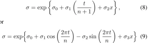
The tree-based threshold selection method is applied to the simulated data sets. The excesses of tree-based threshold are modelled by both stationary and non-stationary GP model. Co-variate models are incorporated in the scale parameter of non-stationary GP model such that the scale parameter is either
σ= exp
σ0+σ1
t
n+ 1
+σ2x
, (8)
or
σ= expnσ0+σ1cos
2πt
n
−σ2sin
2πt
n
+σ3x
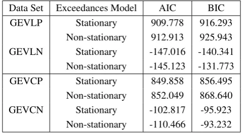
o (9) where Eq. (8) is for data set with linear trend while Eq. (9) is for data set with a cyclic trend. The performance of the fitted stationary GP and non-stationary GP models are compared us-ing Akaike Information Criterion (AIC) and Bayesian Informa-tion Criterion (BIC). The AIC and BIC values are shown in Ta-ble 3. TaTa-ble 3 shows that the AIC and BIC values of stationary model fitted to the tree-based threshold exceedances for simu-lated data with positive shape parameters are smaller compared to the non-stationary model. For simulated data with negative shape parameter, both AIC and BIC show a negative values indicates less information loss than a positive values. Com-parison between stationary and non-stationary models shows that, in overall, the AIC and BIC values are smaller for station-ary than non-stationstation-ary therefore favor the stationstation-ary model in modelling the tree-based threshold exceedances. This conclude that regression tree method are able to produce most stationary data within the cluster, hence simpler model can be fit into the threshold exceedances.
Table 3. The AIC and BIC values for stationary GP and non-stationary GP models.
Data Set Exceedances Model AIC BIC
GEVLP Stationary 909.778 916.293
Non-stationary 912.913 925.943
GEVLN Stationary -147.016 -140.341
Non-stationary -145.123 -131.773
GEVCP Stationary 849.858 856.495
Non-stationary 852.049 868.640
GEVCN Stationary -102.817 -95.923
Non-stationary -110.466 -93.232
Mean Squared Error (RMSE) and coefficient of determination (R2) values are used to compare the performance of both
[image:5.595.59.276.415.548.2]meth-ods. Result in Table 4 shows that the RMSE values for tree-based threshold method are smaller compared to the standard method except for GEVLP. However, the value of RMSE for tree-based threshold method is quite close to the RMSE for standard method with covariates model indicating that these two methods are comparable with the advantage to the tree-based threshold method because of less parameter has to be estimated. Moreover, the R2 values for tree-based threshold selection method is closer to 1 compared to standard method.
Table 4.The RMSE and R2values for threshold exceedances model.
Data set Exceedances Model RMSE R2
GEVLP Tree-based 3.520 0.960
Standard 2.171 0.971
GEVLN Tree-based 0.287 0.998
Standard 0.647 0.953
GEVCP Tree-based 3.700 0.973
Standard 4.890 0.910
GEVCN Tree-based 0.370 0.999
Standard 0.516 0.933
5
API Data Analysis
In this section, the proposed tree-based threshold selection method is applied to daily maxima of API and covariates PM10,
O3, SO2, NO2and CO data as described in Section 2. Table 5
shows the percentage of missing values for the data sets. As the percentage of missing values in several covariate are quite high, we use the Full Conditional Specification technique to impute the missing data. In this technique, each incomplete variable is imputed by a separate model. The imputation is done using micepackage in Rsoftware and the algorithm is completely discussed in [15]. The descriptive statistics for API data and the covariates after the imputation is given in Table 6. From Table 6, the highest API recorded during the study period is 257 which falls in very unhealthy level.
We develop the regression tree for API and covariates data us-ing procedure discussed in Section 3.2 withδ = 0.000083.
Table 5.Percentage of missing values for API and covariates data.
Variable API PM10 O3 SO2 NO2 CO
Percentage 0.16 0.68 6.04 20.53 20.58 24.91 Table 6.Descriptive statistics for API and covariates data.
Variable Mean Median Minimum Maximum Variance
API 56.739 54 18 257 39.244
PM10 51.084 45.306 9.129 389.77 842.942
O3 0.032 0.024 0 0.131 0.0009
SO2 0.004 0.003 0 0.358 5.628×10⁻⁵
NO2 0.028 0.027 0 0.202 0.0001
CO 1.289 1.226 0.025 7.412 0.243
The regression tree shown in Figure 2 produce 71 clusters with O3and PM10become a dominant covariates that split the
API data. For each resulted clusters, we set 95th percentile threshold producing a covariate-varying threshold known as tree-based threshold as shown in Figure 3. The exceedances of tree-based threshold is then modelled by both stationary and non-stationary GP model. Since PM10and O3are the dominant
pollutants that split the API data, we consider these pollutants in modelling the tree-based threshold excesses of API data for non-stationary GP model. Study by [8] also shows that PM10
and O3are the dominants pollutants that affect the variation in
API data. The covariates model is incorporated in the scale pa-rameter of GP model such thatσ= exp(σ0+σ1O3+σ2PM10)
where the exponential function is used to ensure that the posi-tivity ofσis respected for all values of PM10and O3. Table 7
shows the parameter estimates of stationary and non-stationary GP model fitted to the tree-based threshold excesses API data. From Table 7, both models have positive shape parameter indi-cates that the distribution of tree-based threshold exceedances for API data is unbounded. The performance of the stationary and non-stationary GP model fitted to the tree-based threshold exceedances are evaluated using AIC and BIC. The AIC and BIC values are shown in Table 8. Based on Table 8, the AIC and BIC values are smaller for stationary GP model compared to non-stationary model, which conclude that modelling tree-based threshold excess with stationary GP model produce less information loss. Hence, this method provide much simpler model to explain the variation in API data. The goodness-of-fit (GoF) of the stationary GP model is tested using Anderson-Darling (AD) test and Cramer von Misses (CVM) test. The
p-values of the GoF tests shown in Table 9 indicates that the stationary GP model fit the tree-based threshold exceedances of API data well.
Table 7.Parameter estimates of stationary and non-stationary GP model fitted to the tree-based threshold exceedances of API data.
Exceedances Model σ0 σ1 σ2 ξ
Stationary 3.313380 - - 0.276766
Non-stationary 1.109091 -0.129322 0.002481 0.224365
We also compare the tree-based threshold selection method with the standard method using RMSE and R2. A constant
pro-Figure 2.Regression tree for API data.
Figure 3.API data and tree-based threshold line obtained from regression tree.
Table 8.AIC and BIC values fitted to the tree-based threshold exceedances of API data.
Exceedances Model AIC BIC
Stationary 325.732 330.0808 Non-stationary 328.552 337.2496 Table 9.Thep-values of AD and CVM tests for stationary GP model.
AD test CVM test 0.8686 0.8513
duces less error and better at forecasting predicted values. This result also supported by value of R2which is much closer to 1
compared to the R2value for standard method. Table 10.RMSE and R2values applied on API data.
Method RMSE R2
Tree-based 5.262 0.995 Standard 163.258 0.919
6
Conclusion
In this paper, a new and simple method for threshold selec-tion for the GPD in the presence of covariate is presented. The method uses regression tree to partition the data sets into ap-proximately stationary series. The excesses of the tree-based threshold is shown to be better fitted with stationary GP model compared to non-stationary GP model producing much simpler model to explain the variation in data sets. Comparison made with the standard method shows that the proposed tree-based
threshold is much better in terms of producing less error and better at forecasting values. In modelling the API data, the tree-based threshold is sufficiently enough to produce a stationary threshold exceedances so that much simpler model could be fitted in order to explain the variation in API data. In practice, our method can be seen as an additional tool that complements existing threshold selection methods.
Acknowledgment
The authors would like to thank the Department of Environ-ment, Malaysia for providing the air quality data. This work was funded by the Geran Putra - Inisiatif Pensyarah Muda, Uni-versiti Putra Malaysia (GP-IPM/2016/9513100)
REFERENCES
[1] Abdullah, M. Z. & Alias, N. A. (2018). Variation of PM10
and heavy metals concentration of suburban area caused by haze episode. Malaysian Journal of Analytical Sciences, 22(3):508–513.
[2] Al-Dhurafi, N. A., Masseran, N., Zamzuri, Z. H., & Razali, A. M. (2018). Modeling unhealthy air pollution index using a peaks-over-threshold method.Environmental Engineering Sci-ence, 35(2), 101-110.
[3] Coles, S., Bawa, J., Trenner, L., & Dorazio, P. (2001).An in-troduction to statistical modeling of extreme values(Vol. 208). London: Springer.
[4] Roberts, E. M. (1979a). Review of statistics of extreme values with applications to air quality data, Part I, Review.Journal of the Air Pollution Control Association, 29: 632-637.
[5] Roberts, E. M. (1979b). Review of statistics of extreme values with applications to air quality data, Part II, Applications. Jour-nal of the Air Pollution Control Association, 29: 733-740.
[6] Amin, N. A. M., Adam, M. B., & Aris, A. Z. (2015). Extreme value analysis for modeling high PM10level in Johor Bahru.
Jurnal Teknologi, 76(1).
[7] Masseran, N., Razali, A. M., Ibrahim, K., & Latif, M. T. (2016). Modeling air quality in main cities of peninsular malaysia by us-ing a generalized pareto model.Environmental monitoring and assessment, 188(1):65.
[8] Al-Dhurafi, N. A., Masseran, N., Zamzuri, Z. H., & Razali, A. M. (2018). Modeling unhealthy air pollution index using a peaks-over-threshold method.Environmental Engineering Sci-ence, 35(2):101–110.
[9] Northrop, P. J., & Jonathan, P. (2011). Threshold modelling of spatially dependent non-stationary extremes with application to hurricane-induced wave heights.Environmetrics, 22(7), 799-809.
[11] Pickands III, J. (1975). Statistical inference using extreme order statistics.the Annals of Statistics, 3(1), 119-131.
[12] Davison, A. C., & Smith, R. L. (1990). Models for exceedances over high thresholds.Journal of the Royal Statistical Society: Series B (Methodological), 52(3), 393-425.
[13] Breiman, L., Friedman, J. H., Olshen, R. A. & Stone, C. J. (1984).Classification and Regression Trees. London: Chapman and Hall.
[14] Eastoe, E. F., & Tawn, J. A. (2009). Modelling non-stationary extremes with application to surface level ozone.Journal of the Royal Statistical Society: Series C (Applied Statistics), 58(1), 25-45.