General Classical Electrodynamics
Koen J. van Vlaenderen
EthergyB.V,Research,Hobbemalaan10,1816GDAlkmaar,NorthHolland,TheNetherlands InstituteforBasicResearch,P.O.Box1577,PalmHarbor,FL34684U.S.A.
Copyright c2016 by authors, all rights reserved. Authors agree that this article remains permanently
open access under the terms of the Creative Commons Attribution License 4.0 International License
Abstract
Maxwell’s Classical Electrodynamics (MCED) suffers several inconsistencies: (1) the Lorentz force law of MCED violates Newton’s Third Law of Motion (N3LM) in case of stationary and divergent or convergent current distri-butions; (2) the general Jefimenko electric field solution of MCED shows two longitudinal far fields that are not waves; (3) the ratio of the electrodynamic energy-momentum of a charged sphere in uniform motion has an incorrect factor of 43. A consistent General Classical Electrodynamics(GCED) is presented that is based on Whittaker’s reciprocal force law that satisfies N3LM. The Whittaker force is expressed as a scalar magnetic field force, added to the Lorentz force. GCED is consistent only if it is assumed that the electric potential velocity in vacuum, ’a’, is much greater than ’c’ (a c); GCED reduces to MCED, in case we assume a = c. Longitudinal electromagnetic waves and superluminal longitudinal electric potential waves are predicted. This theory has been verified by seemingly unrelated experiments, such as the detection of superluminal Coulomb fields and longitudinal Amp`ere forces, and has a wide range of electrical engineering applications.
Keywords
Classical Electrodynamics, Longitudinal Amp`ere Force, Scalar Fields, Longitudinal Electric Waves, Superluminal Velocity, Energy Conversion1
Introduction
An alternative to Maxwell’s [1, 2] Classical Electrodynam-ics (MCED) theory is presented, called General Classical Electrodynamics(GCED), that is free of inconsistencies. For the development of this theory we make use of the fundamen-tal theorem of vector algebra. The proof of this fundamenfundamen-tal theorem is based on the three dimensional delta functionδ(x) and the sifting property of this function, see (1.1 – 1.2):
δ(x) = −1 4π∆
1
|x|
(1.1)
F(x) = Z
V0
F(x0)δ(x−x0) d3x0 (1.2)
The fundamental theorem of vector algebra is as follows: a vector function F(x) can be decomposed into two unique vector functions Fl(x) and Ft(x), such that
F(x) = Fl(x) +Ft(x) (1.3)
Fl(x) = − 1
4π∇
Z
V0
∇0·
F(x0)
|x−x0| d
3
x0 (1.4)
Ft(x) = 1 4π∇×
Z
V0
∇0×F(x0)
|x−x0| d
3
x0 (1.5)
The lowercase subindexes ’l’ and ’t’ will have the meaning oflongitudinalandtransversein this paper. The longitudinal vector functionFl is curl free (∇×Fl =0), and the
trans-verse vector functionFt is divergence free (∇·Ft= 0). We
assume thatFis well behaved (Fis zero if|x|is infinite). Let us further introduce the following notations and definitions.
ρ Net electric charge density, in C/m3
J=Jl+Jt Net electric current density, in A/m2
Φ Net electric charge (scalar) potential, in V
A=Al+At Net electric current (vector) potential,
in V·s/m
EΦ=−∇Φ Electric field, in V/m
EL=−∂tAl Field induced divergent electric field ET=−∂tAt Field induced rotational electric field
BΦ=−∂tΦ Field induced scalar field, in V/s
BL=−∇·Al Scalar magnetic field, in T = V·s/m2 BT =∇×At Vector magnetic field, in T = V·s/m2
φ020µ0 Polarizability of vacuum, in F·s2/m3
µ0 Permeability of vacuum:4π10−7H/m
(x, t) = (x, y, z, t) Place and time coordinates
∂t=
∂
∂t Partial time differential ∇=
∂ ∂x,
∂ ∂y,
∂ ∂z
Del operator
∆ =∇ · ∇ Laplace operator
∆Φ =∇·∇Φ, ∆A=∇∇·A− ∇×∇×A
The permittivity, permeability and polarizability of vacuum are constants. The charge- and current density distributions, the potentials and the fields, are functions of place and not always functions of time. Time independent functions are calledstationaryorstaticfunctions. Basically there are three types of charge-current density distributions:
A. Current free charge J=0 B. Stationary currents ∂tJ=0
1. closed circuit ∂tJ=0 ∧ ∇·J=0
2. open circuit ∂tJ=0 ∧ ∇·J6=0
C. Time dependent currents ∂tJ6=0
The charge conservation law (also called ’charge continuity’) is true for all types of charge-current density distributions:
∂ρ
∂t +∇·J = 0 (1.6) The physics of current free charge density distributions is calledElectrostatics(ES): ∂tρ=−∇·0= 0. The physics
of stationary current density distributions (∂tJ=0) is called
General Magnetostatics(GMS). A special case of GMS are
divergence free current distributions (∇ ·J = 0), and this is widely calledMagnetostatics(MS) in the scientific educa-tional literature. In case of Magnetostatics, the charge density distribution has to be static as well: ∂tρ=−∇·J= 0, such
that the electric field and the magnetic field are both static. The Maxwell-Lorentz force law satisfies Newton’s third law of motion (N3LM) in case of Electrostatics and Magne-tostatics, however, this force law violates N3LM in case of General Magnetostatics. A violation of N3LM means that momentum is not conserved by GMS systems, for which there is no experimental evidence! This remarkable inconsis-tency in classical physics is rarely mentioned in the scientific educational literature.
This is not the only problematic aspects of MCED. Jefi-menko’s electric field expression that is derived from MCED theory, shows two longitudinal electric field terms that do not interact by induction with other fields, therefore these electric fields cannot be field waves and nevertheless these electric fields fall off in magnitude by distance, as far fields, which is inconsistent. A third inconsistency is the problematic 43 fac-tor in the ratio of the electric energy and the electromagnetic momentum of a charged sphere. In the next sections we de-scribe these related inconsistencies of MCED theory in more detail, and how to resolve them.
2
General Magnetostatics
LetJ(x)be a stationary current distribution. The vector potentialA(x)at place vectorxis given by:
A(x) = µ0 4π
Z
V0 J(x0)
r d
3
x0 (2.1)
r = x−x0
r = |x−x0|
Since ∂tA = 0 for stationary currents, the electric field
equalsE=EΦ=−∇Φ, such that the Gauss law for General
Magnetostatics is given by ∇·EΦ(x, t) =
1
0
ρ(x, t) (2.2)
The magnetostatic vector field BT(x) is defined by
Biot-Savart’s law as follows:
BT(x) = ∇×At(x) = ∇×A(x)
= −µ0
4π
Z
V0
J(x0)× ∇
1
r
d3x0
= µ0 4π
Z
V0 1
r3
J(x0)×r
d3x0 (2.3)
The magnetic field is indeed static, since the current density is stationary. From the continuity of charge (1.6), and (2.2), it follows that Jl =−0∂t(EΦ), hence the Amp`ere law for
General Magnetostatics is as follows: ∇×BT−0µ0
∂EΦ
∂t = µ0J (2.4)
2.1
The Lorentz force
The magnetic force density, fT(x), that acts transversely
on current density J(x)at placex, is given by:
fT(x) =J(x)×BT(x)
=µ0 4π
Z
V0 1
r3J(x)×
J(x0)×r d3x0
=µ0 4π
Z
V0 1
r3
h
J(x)·r
J(x0) −
J(x0)·J(x) rid3x0
=µ0 4π
Z
V0 fT(x,x
0
) d3x0 (2.5)
This is the Lorentz force density law for Magnetostatics; it is assumed that the electric force densities are negligible. Notice that the integrand is non-reciprocal: fT(x,x0) 6=
−fT(x0,x), and thatrchanges into−rby swappingxand x0. This means that the Lorentz force law agrees with N3LM, but only if one calculates the total force onclosed on-itself
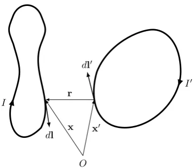
current circuits (magnetostatics is usually defined for diver-gence free currents only), which is proven as follows. Consider two non-intersecting and closed current circuitsC andC0, that carry the stationary electric currentsI andI0, see figure 1. The currentsI andI0 are equal to the surface integral of the current density over a circuit line cross sec-tion of respectively circuitsCandC0. The total force acting on circuitCis a double volume integral of the Lorentz force density. We assume that the currents inC andC0 are con-stantfor each circuit line cross section, therefore we replace the double volume integral by a double line integral over the circuitsCandC0, in order to determine the force,FC, acting
I
I0
dl
dl0
r
x x0
[image:3.595.65.261.64.234.2]O
Figure 1.Closed stationary current circuits
FC =−
µ0II0
4π
I
C I
C0
dl×(dl0× ∇
1
r
)
=−µ0II 0
4π
I
C0 I
C h
(dl· ∇
1
r
)dl0 − (dl·dl0)∇
1
r
i
= µ0II
0
4π
I
C I
C0
(dl·dl0)∇
1
r
(2.6)
This is Grassmann’s [3] force law for closed current circuits. Since the curl of a gradient is zero, the first integral disap-pears, see (2.6) after the first derivation. The final integral after derivation step 2 has a reciprocal integrand, such that the force acting on circuitC0is the exact opposite of the force acting on circuitC(FC=−FC0), in agreement with N3LM.
Fubini’s theorem is applicable in derivation step 1 (switching the integration order in the first integral), since it is assumed the circuitsCandC0do not intersect.
The standard literature on Classical Electrodynamics usu-ally defines Magnetostatics as the physics of stationary and
divergence free(closed circuits) electric currents. For ex-ample, the Feynman lectures [4, Vol II,§13.4] describe that Magnetostatics is based on equation∇×BT =µJ, such that
Magnetostatic current is divergence free, such that the elec-tric field is also static, and such that charge density is con-stant in time:∇·J= 0 =∂tρ. R. Feynman further suggests
that a Magnetostatic circuit may contain batteries or genera-tors that keep the charges flowing, however, an electric bat-tery delivers an electrical current only if the batbat-tery’s charge density changes in time. A generator of stationary current is for example Faraday’s homopolar disk generator, which can be included in a stationary closed current loop. One has to measure the forceFCon the entire closed circuit that
in-cludes the generator as well, while the generator is externally driven with constant speed. Such a magnetostatic force ex-periment has yet to be done. J. D. Jackson’s [5] third edition of Classical Electrodynamics postulates without proof that ∇ ·J = 0 = ∂tρ(charge density is time-independent
any-where in space, see after equation 5.3) before Jackson treats the laws of magnetostatics. D. J. Griffiths’ [6] treatment of magnetostatics is likewise: ”stationary electric currents are such that the density of charge is constant anywhere”, which means that stationary currents that are divergence free. A. Altland [7] defined ’statics’ as ’static electric fields and static magnetic fields’, and again this implies that∇·J= 0 =∂tρ.
Etc ...
It is not at all straightforward to find practical examples of a measured force exerted on a stationary and perfectly closed-on-itself current circuit. The Meisner effect might be such an example: a free falling permanent magnet approaches a su-perconductor, which induces a closed-circuit current in the superconductor. The magnet falls until the induced currents and magnetic field of the superconductor perfectly opposes the field of the magnet, which causes the magnet to levitate, and from that moment on the superconductor current is sta-tionary and divergence free. However, we cannot measure the ”electric current” of the floating permanent magnet, in order to derive a magnetostatics force law. An electrically charged rotating object may represent a closed-circuit stationary cur-rent, however, it seems impractical to measure forces on such objects while keeping the rotation speed constant during the measurements. Amp`ere force experiments with two coils that conduct stationary currents have been performed frequently in history. A coil with several windings gives the impression of a perfectly closed current loop, however, this is only true approximately.
Many stationary current experiments have been conducted to measure the Amp`ere force on a circuit that isnot closed-on-itself, see figure 2.
∂tρ <0
∂tρ >0 ∂tρ >0
∂tρ <0 O
I I
I0 I0 dl
dl0
x x0
[image:3.595.308.528.368.481.2]r
Figure 2.Open stationary current circuits
One can perform such experiments by applying two sliding contacts in order to enable a rotation- or translation motion of a circuit part that is non-closed, such that a force can be mea-sured on just this movable circuit part. Faraday’s homopolar disk motor is an example of this principle. Stefan Marinov’s [8] Siberian Coliu motor is another example of a two sliding contacts motor, driven by a stationary current. Another type of non-closed current circuits make use of light weight mov-able batteries, such that sliding contacts can be avoided. This shows that the condition∇·J= 0 =∂tρ, as well as the
condi-tions∇×B=µJand∂tE=0, are artificial and superfluous
for force experiments on stationary electric currents. A possible reason for reducing General Magnetostatics to Magnetostatics by means of the false assumption that sta-tionary currents are divergence free in general, is to obscure mathematically the violation of N3LM by the Grassmann force law [9], and also by the more general Lorentz force law. General Magnetostatics may be consistent with Classi-cal Mechanics, if the Lorentz force law is replaced by another force law that satisfies N3LM.
2.2
The Whittaker force
Amp`ere’s force law by E. T. Whittaker [10, p.91], resulted in the following Whittaker force law,
FC=
µ0II0
4π
Z
C Z
C0 1
r3
h
(dl0·r)dl+ (dl·r)dl0−(dl·dl0)r)i (2.7)
that is equal to Grassmann’s force law (2.6), except for the additional term(dl0·r)dl. Both force laws predict the same force acting on closed on-itself circuits, since the line integral of the additional term over a closed circuit disappears as well. However, Whittaker’s force law is reciprocal (FC =−FC0),
also for non-closed circuits, and satisfies N3LM for General Magnetostatics.
By means of the following functions, defined as follows,
BL(x) = −∇·Al(x) = − ∇·A(x)
= −µ0 4π
Z
V0
J(x0)· ∇ 1
r
d3x0
= µ0 4π
Z
V0
1 r3
J(x0)·rd3x0 (2.8)
fL(x) = J(x)BL(x) (2.9)
we generalize Whittaker’s force law as a double volume inte-gral of field force densities, see [11, equation 13], and [12]:
Z
V
h
fL(x) +fT(x)
i d3x =
Z
V
h
J(x)BL(x) + J(x)×BT(x)
i d3x =
µ0
4π Z
V
Z
V0
1 r3
J(x0)·r
J(x) +
J(x)·r
J(x0)−
J(x0)·J(x)
r
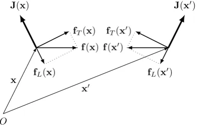
d3x0d3x (2.10) This double volume integral of force densities satisfies N3LM for stationary current densities in general, since the integrand is reciprocal. The additional force density,fL, is
called thelongitudinal Amp`ere force density, which balances the transverse Amp`ere force density, fT, such that the
to-tal Amp`ere force density f(x) = fL(x) +fT(x) satisfies f(x) =−f(x0), see figure 3.
O
J(x) J(x0)
x
x0
f(x)
fL(x)
fT(x)
fL(x0) f(x0)
[image:4.595.77.280.615.749.2]fT(x0)
Figure 3.Total Amp`ere force density
It is obvious that the scalar functionBLis aphysical field
that mediates an observable Amp`ere force, just like the vec-tor magnetic fieldBT, and therefore it is called thescalar
magnetic field[13].
2.3
The Lorenz condition
By means of (1.1), (1.2) and (2.3), (2.8), we derive the following equations:
∇BL(x) +∇×BT(x) =−∆A(x) =µ0J(x) (2.11)
∇BL(x) =−∇∇·Al(x) =µ0Jl(x) (2.12)
∇×BT(x) =∇×∇×At(x) =µ0Jt(x) (2.13)
The following GMS condition follows from (2.4), (2.11) and (3.1), and is known as the Lorenz condition [14]:
∇(BL+0µ0BΦ) = 0 (2.14)
This GMS condition is not a free to choose ”gauge” condi-tion. If the scalar functionBLhas the meaning of a physical
field, then Lorenz’s condition shows that the scalar function BΦalso has the meaning of a physical field. So far we have
shown a consistent GMS theory in agreement with classical mechanics.
3
General CED
We continue to develop the theory of General CED that describes the physics of time dependent currents, taking into account the physical scalar fieldsBL,BΦ and (2.2), (2.12)
and (2.13).
3.1
General field induction
The field equations that describe the induction of sec-ondary fields by primary time dependent fields, follow di-rectly from the field definitions and the fact that the operators ∇,∇· and∇× commute with∂t:
∇BΦ−
∂EΦ
∂t = − ∇ ∂Φ
∂t + ∂(∇Φ)
∂t = 0 (3.1) ∇·EL−
∂BL
∂t = − ∇· ∂Al
∂t +
∂(∇·Al)
∂t = 0 (3.2) ∇×ET+
∂BT
∂t = − ∇× ∂At
∂t +
∂(∇×At)
∂t = 0 (3.3) This is the generalization of Faraday’s [15] law of induction, see (3.3). A curl-free electric fieldELis induced by a time
varying scalar magnetic field BL, see (3.2), which is
simi-lar to the Faraday induction of a divergence-free electric field
ET. Equation (3.2) will be calledNikolaev’s [13] law of
elec-tromagnetic induction, after G.V. Nikolaev.
Electric fields are sourced by static charges and induced by time varying vector- and scalar magnetic fields. According to the superposition principle, a superimposed electric field is defined asE=EΦ+EL+ET =−∇Φ−∂tA. Notice
thatEl=EΦ+ELand thatEt=ET.
3.2
The essence of Maxwell’s CED
Maxwell’s famous treatise on electricity and magnetism does not include the definitions of the fields BL and BΦ,
and does not include Nikolaev’s induction law. However, Maxwell defined the superimposed electric field as E =
EΦ+EL+ET, without explaining the induction of the
sec-ondary field EL by a time varying primary field BL. We
cannot just assume the existence of fieldELwithout
be defined asE = EΦ+ET, according to Ockham’s
ra-zor. This simple definition reduces MCED to its experimen-tal essence, and fixes the indeterminacy (gauge freedom) of the charge- and current potentials: the electric fieldEΦ+ET
is not invariant with respect to the ”gauge” potential transfor-mation. The following field equations describe the essence of Maxwell’s CED:
EΦ+ET = E (3.4)
∇·E = ∇·EΦ =
1
0
ρ (3.5)
∇×E = ∇×ET = −
∂BT
∂t (3.6) ∇×BT − 0µ0
∂(EΦ+ET)
∂t = µ0J (3.7) Completed with the Lorentz force law, this theory is called
Special Classical Electrodynamics(SCED). From the charge continuity law follows the next ’displacement current’ equa-tion:
−0
∂EΦ
∂t = Jl (3.8) Substraction of (3.8) from (3.7) gives the following equation.
∇×BT−0µ0
∂ET
∂t = µ0Jt (3.9) The presence of Maxwell’s displacement current term 0∂tET in the Maxwell-Amp`ere law (3.7) and in (3.9) does
not follow directly from charge continuity, since this term is divergence free. The addition of this term by Maxwell was an unfounded conjecture, which led to the derivation of the transverse electromagnetic (TEM) wave equations. Maxwell’s conjecture was eventually proven and verified by Hertz’s [16] electromagnetic wave detection experiments.
Rewriting (3.5) and (3.9) in terms of the potentials gives:
−∆Φ = 1
0
ρ (3.10)
0µ0
∂2At
∂t2 +∇×∇×At = µ0Jt (3.11)
The derivation of these ’decoupled’ differential equations for the potentials is independent of gauge conditions and gauge transformations. The indeterminacy (gauge freedom) of the potentials is a direct consequence of Maxwell’s unfounded addition of the fieldEL to the superimposed electric field,
within the context of MCED. These equations have the fol-lowing solutions.
Φ(x, t) = 1 4π0
Z
V0
ρ(x0, t)
r d
3
x0 (3.12)
At(x, t) = µ0 4π
Z
V0
Jt(x0, tc)
r d
3
x0 (3.13)
r = |x−x0| c= √1 0µ0
tc = t−
r
c (3.14)
The net charge potentialΦis instantaneous at a distance. The net current potentialAt is retarded with time interval r/c,
relative to current potential sources at a distancer. We derive general field solutions, similar to the Jefimenko’s fields, from the potential functions 3.12 and 3.13, and definition 3.4:
BT(x, t) =
µ0
4π
Z
V0
Jt(x0, tc)×r
r3 +
˙
Jt(x0, tc)×r
cr2
d3x0
(3.15)
E(x, t) = 1 4π0
Z
V0
ρ(x0, t)r
r3 −
˙ Jt(x0, tc)
c2r
d3x0 (3.16)
Jefimenko’s general fields are derived from MCED, and are the following expressions:
BT(x, t) =
µ0
4π
Z
V0
Jt(x0, tc)×r
r3 +
˙
Jt(x0, tc)×r
cr2
d3x0
(3.17)
E(x, t) = 1 4π0
Z
V0
ρ(x0, tc)r
r3 +
˙
ρ(x0, tc)r
cr2
−J˙l(x 0
, tc)
c2r −
˙ Jt(x0, tc)
c2r
d3x0 (3.18)
Jackson [17] proved that Jefimenko’s field expressions do not depend on the choice for gauge condition. Notice that Jefi-menko’s magnetic field is expressed in terms of the diver-gence free current density, Jt. The second term and third
term of the integrand of (3.18) are longitudinal electric far fields that fall off in magnitude by r. Since far fields are field waves that can only exist as two fields that induce each other in turn, these two far field terms represent an inconsis-tency, since MCED does not define the two other fields that mutually induce the two longitudinal electric far fields that occur in Jefimenko’s electric field expression. The two miss-ing fields prove to beBΦandBL, see§3.3. We call this the
far field inconsistencyof MCED.
SCED theory is manifestly far field consistent, since (3.15) and (3.16) only show the two far fields of the transverse elec-tromagnetic wave. SCED is a consistent theory as special case of GCED with the condition Jl = 0. If we assume Jl = 0, then the second and third term in the integrand
of (3.18) disappear, and in that case MCED and SCED are equal, except that the first integrand term of (3.18) is re-tarded, where the first integrand term of (3.16) is instanta-neous. SCED and MCED describe the same physical effects in essence, if we ignore for a moment those experiments that determine the velocity of the near electric field.
3.3
General displacement terms and
general field waves
We combine GMS with SCED in order to derive a consis-tent GCED. This theory should treatJlandρas the sources
of fieldsBL, BΦ andEL, and should define the
superim-posed electric field asE=EΦ+EL+ET. We already
gen-eralized Faraday’s field induction law in§3.1, and now we generalize Maxwell’s conjectural term0∂tET, by adding a
displacement charge term φ0∂tBΦto(3.5) and a second
dis-placement current term λ0∂tELto (2.12):
∇·EΦ−
φ0
0
∂BΦ
∂t = φ0
0
∂2Φ
∂t2 − ∇·∇Φ =
1
0
ρ (3.19)
∇BL−λ0µ0
∂EL
∂t =λ0µ0 ∂2A
l
∂t2 − ∇∇·Al=µ0Jl (3.20)
∇×BT−0µ0
∂ET
∂t =0µ0 ∂2A
t
∂t2 +∇×∇×At=µ0Jt
The constant,φ0, is called theelectric polarizabilityof
vac-uum, and its unit isF s2m−3. In case of a stationary current potential (∂tA = 0), the GCED equations (3.20–3.21)
re-duce to the GMS equations (2.12–2.13), such that GCED will obey N3LM for open circuit stationary current distributions, by deducing the correct force theorem later on. The follow-ing inhomogeneous field wave equations can be derived from (3.1–3.3) and (3.19–3.21).
φ0
0
∂2E Φ
∂t2 − ∇∇·EΦ = −
1 0
∇ρ (3.22) φ0
0
∂2B Φ
∂t2 − ∇·∇BΦ = −
1 0
∂ρ
∂t (3.23)
λ0µ0
∂2EL
∂t2 − ∇∇·EL = −µ0
∂Jl
∂t (3.24) λ0µ0
∂2B
L
∂t2 − ∇·∇BL = −µ0∇·Jl (3.25)
0µ0
∂2ET
∂t2 +∇×∇×ET = −µ0
∂Jt
∂t (3.26) 0µ0
∂2B
T
∂t2 +∇×∇×BT = µ0∇×Jt (3.27)
These wave equations describe the Transverse Electromag-netic (TEM) wave and two types of longitudinal electric waves. One type of longitudinal electric wave is expressed only in terms of the electric charge potentialΦ, so it is not in-duced by electric currents, see (3.22–3.23). It will be called a Φ-wave. The second type of longitudinal electric wave is associated with the curl free electric current potential, see (3.24–3.25), and it will be called aLongitudinal Electromag-netic (LEM) wave. The following notations for the phase velocities of these wave types is used.
a = r
0
φ0
, b = r
1 λ0µ0
, c = r
1 0µ0
(3.28)
Initially we assume that the values of these phase velocities are independent constants, and that is why we introduced the new constantsλ0andφ0. The additional theoretical
predic-tion of the LEM wave and theΦ-wave are testable, as before Maxwell’s TEM wave prediction was tested by Hertz.
3.4
General power- and force theorems
Three power- and force laws can be derived that are asso-ciated with theΦ-wave, the LEM wave and the TEM wave. The power- and force law for theΦ-wave fieldsBΦandEΦ
are derived from (3.1) and (3.19):
−ρBΦ=
φ0
2
∂B2Φ
∂t + 0
2
∂EΦ2
∂t −0∇·(BΦEΦ) (3.29) ρEΦ=φ0(∇BΦ)BΦ +0(∇·EΦ)EΦ −φ0
∂(BΦEΦ)
∂t
(3.30)
The power- and force law for the LEM wave fieldsBL and ELare derived from (3.2) and (3.20l):
−EL·Jl= 1 2µ0
∂BL2
∂t + λ0
2
∂EL2
∂t −
1
µ0
∇·(BLEL) (3.31)
BLJl= 1
µ0
(∇BL)BL +λ0(∇·EL)EL
−λ0
∂(BLEL)
∂t (3.32)
The power- and force law for the TEM wave fieldsBT and ET are derived from (3.3) and (3.21):
−ET·Jt= 1 2µ0
∂BT2
∂t + 0
2
∂ET2
∂t
− 1 µ0
∇·(BT×ET) (3.33)
BT×Jt= 1
µ0
BT× ∇×BT +0ET× ∇×ET
−0
∂(BT×ET)
∂t (3.34)
Similar energy flux vectors as Poynting’s vector for the TEM wave,−BT ×ET, can be defined for theΦ-wave: BΦEΦ
(see the last term in (3.29) and in (3.30), and for the LEM wave: BLEL (see the last term in (3.31) and in (3.32). For
very small values ofφ0, theΦ-wave contribution to
momen-tum changebecomes very small as well, and yet theΦ-wave contribution topower fluxmight be substantial!
Notice that the fields in these power- and force theorems are not superimposed fields. The most general power- and force theorems should be expressed in terms of superimposed fields, and these are defined as follows:
E = EΦ + EL + ET (3.35)
E∗ = 1
c2EΦ +
1
b2EL +
1
c2ET (3.36)
B = 1
c2BΦ + BL (3.37)
B∗ = 1
a2BΦ + BL (3.38)
The field equations (3.19–3.21) are rewritten in terms of these fields.
∇·E −∂B ∗
∂t =
1
0
ρ (3.39)
∇B +∇×BT −
∂E∗
∂t = µ0J (3.40) General power- and force theorems follow from (3.39) and (3.40):
−E·J−c2Bρ= 1
µ0
[E·∂E ∗
∂t +BT· ∂BT
∂t +B ∂B∗
∂t ]
− 1 µ0
∇·(BT×E +BE) (3.41)
ρE + J×BT + (
0
λ0
Jl+Jt)B∗=
0(∇·E)E +
1
µ0
(∇×E)×E∗ +
1
µ0
(∇B+∇×BT)×BT +
(0∇BΦ+
0
λ0µ0
∇BL+ 1
µ0
∇×BT)B
∗ −
0
∂(EB∗)
∂t −
1
µ0
∂(E∗×BT)
In (3.42) the expression(λ0
0Jl+Jt)has to equalJin
or-der to deduce the force law of (2.10) that satisfies N3LM. Therefore, the following condition is generally true: λ0 =
0 (b=c). Applying this condition, the general power- and
force theorems become (ifb=cthenE∗= c12E):
−E·J−c2Bρ=
0
2
∂E2 ∂t +
1 2µ0
∂BT2
∂t + B µ0
∂B∗ ∂t
− 1 µ0
∇·(BT×E +BE) (3.43)
ρE + J×BT + JB∗=
0((∇·E)E + (∇×E)×E) +
1
µ0
(∇B+∇×BT)×BT +
1
µ0
(∇B+∇×BT)B∗ −
0
∂(EB∗ + E×BT)
∂t (3.44)
From the law of charge continuity and the two scalar field wave equations (see (3.23) and (3.25), and also apply λ0 =
0), the following scalar field condition is derived for GCED:
1
c2
∂2B∗
∂t2 − ∇·∇B = 0 (3.45)
In case of general magnetostatics, the scalar fields are in-dependent of time, and (3.45) is reduced to ∇ · ∇B = 0, which is fulfilled by Lorenz’s condition (B = 0), see also (2.14). IfB = 0thenBΦ = −c2BL, andB∗ is expressed
as B∗ = (1−c2/a2)BL. In case of general
magnetostat-ics, we also have E = EΦ, so the power theorem and the
force theorem forGeneral Magnetostaticsare the following two equations:
−EΦ·J =
0
2
∂EΦ2
∂t +
1
µ0
∇·(EΦ×BT) (3.46)
ρEΦ+J×BT+ (1−
c2
a2)JBL =0(∇·EΦ)EΦ
+ 1
µ0
((∇×BT)×BT+ (1−
c2
a2)(∇×BT)BL)
−0
(1−c
2
a2)
∂EΦ
∂t BL+ ∂EΦ
∂t ×BT
(3.47)
This shows that the energy flow carried by stationary currents (for example, from a battery to an energy dissipating resistor [18]) just depend on the ’static’ electric field, EΦ, and the
vector magnetic field,BT, where stationary currents forces
depend also on the scalar magnetic field,BL.
3.5
The Whittaker premise versus the Lorentz
premise
In case of general magnetostatic currents, the density of the scalar magnetic field force must equal fL = JBL,
ac-cording to Whittaker’s force law that satisfies N3LM. Hence, the factor(1−c2/a2)in the GCED force theorem for gen-eral magnetostatics (3.47) must be approximately equal to 1 in order to fulfill N3LM. We conclude that a c must begenerally true, and this is the crux of GCED theory. We will call the assumption, ac, theWhittaker premise, af-ter E.T. Whittaker. This premise should not be confused with
the Coulomb ”gauge” condition, BL = 0. GCED in the
Whittaker premise is called GCED-WP.
The assumption a = c (B∗ = B) will be called the
Lorentz premise, after H.A. Lorentz. This premise should not be confused with the Lorenz ”gauge” condition: B = 0. GCED in the Lorentz premise (GCED-LP) is equivalent with the inconsistent MCED theory, and for this reason the Lorentz premise must befalsein general. This is proven as follows: with a=c(B∗=B), (3.45) becomes:
1
c2
∂2(B)
∂t2 − ∇·∇(B) = 0 (3.48)
This equation implies that the superimposed scalar field ex-ists as a free field wave that isn’t sourced by any charge cur-rent density distribution. If B isn’t sourced by anything, it simply does not exist, then we can set B = 0. It is easy to verify that GCED-LP reduces to MCED, by setting B=B∗= 0.
The scalar fields equation (3.45) is a physical condition
for physical potentials and physical scalar fields, since the Whittaker premise is true. We have shown that MCED, and in particular the confusing indeterminacy of the potentials in the context of MCED can be avoided, by replacing the Lorentz premise for the Whittaker premise. In§4.1 we refer to the experiments that verify the Whittaker premise and falsify the Lorentz premise.
3.6
Retarded potentials and retarded fields
The potentials of GCED-WP are determinate and physi-cal, such that a unique solution of charge-current potentials describes the physics of a particular charge- and current dis-tribution. With a c, andb = c, the scalar- and vector potentials are solutions of the following decoupled inhomo-geneous wave equations:
1
a2
∂2Φ
∂t2 −∆Φ =
1
0
ρ (3.49)
1
c2
∂2A
∂t2 −∆A = µ0J (3.50)
The solutions of these wave equations are the following re-tarded potentials:
Φ(x, t) = 1 4π0
Z
V0
ρ(x0, ta)
r d
3
x0 (3.51)
A(x, t) = µ0 4π
Z
V0
J(x0, tc)
r d
3
x0 (3.52)
r = |x−x0| ta = t−
r
a tc = t− r c
BΦ(x, t) =
1 4π0
Z
V0
−ρ˙(x0, ta)
r d
3
x0 (3.53)
BL(x, t) = µ0 4π
Z
V0
Jl(x0, tc)·r
r3 +
˙
Jl(x0, tc)·r
cr2
d3x0 (3.54)
BT(x, t) = µ0 4π
Z
V0
Jt(x0, tc)×r
r3 +
˙
Jt(x0, tc)×r
cr2
d3x0
(3.55)
E(x, t) = 1 4π0
Z
V0
ρ(x0, ta)r
r3 +
˙
ρ(x0, ta)r
ar2 −
˙ Jl(x0, tc)
c2r
−J˙t(x 0
, tc)
c2r
d3x0 (3.56)
We identify three near field terms, that fall off in magnitude byr2, and six far field terms of theΦ, LEM and TEM waves,
that fall off in magnitude byr, so GCED-WP is far field con-sistent.
Beside Electrostatics and General Magnetostatics, we de-fine two other types of restricted behavior. A charge-current distributions is Quasi Dynamic (QD) if it is assumed that a→ ∞. A charge-current distribution isQuasi Static(QS) if it is assumed that a→ ∞ ∧ c→ ∞. For QD distribu-tions, the retardation of the Coulomb fieldEΦ, and the scalar
potential Φ, is unnoticed (ta = t). The length of the
cir-cuit is much smaller than the wavelength of the farΦ-wave, such that detection of a farΦpotential gradient is impossible: the second term in (3.56) becomes zero. The induction law (3.1) is still needed, since the secondary fieldBΦdoes not
disappear for quasi dynamics. QD is often referred to as ’in-stantaneous action at a distance’ [19]. In case of QS, also the second term in (3.54) and (3.55) become zero. The induction laws for the secondary fieldsELandET are still required for
quasi statics, since the third and fourth term in (3.56) do not disappear.
3.7
The
43problem of MCED
The electrostatic energy,Ee, and the electromagnetic
mo-mentum,pe, of an electron with chargeqe(that is distributed
on the surface of a sphere with classical electron radius,re)
which has a constant speedv, are the following expressions, derived from Maxwell’s CED:
Ee= 1 2
1 4π0
qe2
re
= mec2 (3.57)
pe= 2 3
µ0
4π qe2
re
v = m0ev (3.58)
Notice the following inconsistency: m0e = 43me, which is
known as the 43 problem in the context of MCED.
David E. Rutherford offered a solution to the this problem. His expressions for the electrostatic energy and the electro-magnetic momentum are as follows:
Ee= 1 4π0
q2
e
re
= mec2 (3.59)
pe=
µ0
4π q2
e
re
v = m0ev (3.60)
Firstly, Rutherford [20] proves that the electrostatic energy of the electron is twice that of (3.57), since the work rate,
in order to charge the electron sphere with radiusrewith a
chargeqe, is equal to ∂t(qeΦe) =∂t(qe)Φe + qe∂t(Φe),
and not just equal to ∂t(qe)Φe. If we consider only the
net charge potential, Φ, the GCED power density is equal to ∇Φ·J + ∂t(Φ)ρ. The volume integral of ∇Φ·J equals
Φe∂t(qe). The volume integral of ∂t(Φ)ρ equals ∂t(Φe)qe,
and therefore the energy flow of charging the electron sphere equals ∂t(qeΦe), such that (3.59) also follows from GCED.
This shows that the 43 problem is in fact a 23 problem: an electromagnetic momentum of 13mev is missing.
Sec-ondly, Rutherford [21] derives the electromagnetic momen-tum (3.60) by means of the electromagnetic momenmomen-tum den-sity expression0(EBL+E×BT); the volume integral of the
electromagnetic momentum density 0(EBL) is equal to the
missing 13mevmomentum. The time derivative of this
mo-mentum density expression is exactly the last term of (3.44) in case we apply the Whittaker premise (B∗ = BL), thus
(3.60) follows also from GCED-WP.
Now we haveme=m0ewithout factor43, and this means
that the famous equationE =mc2can be derived from the
non-relativistic GCED-WP theory by evaluating the static en-ergy and the electromagnetic momentum of a charged sphere in uniform motion. The consistent GCED-WP theory does not suffer the 43 problem either.
4
Review of CED experiments
The development of GCED-WP was motivated by Nikola Tesla’s [22, 23] remarkable achievements in electrical en-gineering. Tesla described his long distance electric en-ergy transport system as transmission of longitudinal elec-tric waves, conducted by a single wire or the natural me-dia, including the aether. Mainstream physics predicts that longitudinal electric waves exist as sound waves conducted by material media only. GCED-WP predicts luminal lon-gitudinal electromagnetic waves, and super luminal electric Φ-waves in vacuum as well, hence, for the first time in his-tory Tesla’s observation of a longitudinal aether sound wave is supported by an exact theory. The characteristic ’quarter wave length’ distribution, across the unwound wire length of the secondary coil of Tesla’s transformer device, is hard to ex-plain by conventional electrodynamics theory, where GCED-WP explains this wave type naturally as a LEM wave. A most general review is required for a wide range of CED experi-ments that may verify or falsify the new aspects of GCED-WP theory.
4.1
The superluminal Coulomb field
4.2
General Magnetostatic force experiments
The historic Magnetostatic force experiments carried out by Amp`ere, Gauss, Weber and other famous scientist, are examples ofopen circuit currents. It is certain that batter-ies or very large capacitor banks were used as electric cur-rent sources and curcur-rent sinks that typically showed time varying charge densities and divergent currents at the cur-rent source/sink interface, however, delivered a steady volt-age and a stationary current.
Specific General Magnetostatic experiments such as Amp`ere’s historic hairpin experiment, demonstrate the exis-tence of the longitudinal Amp`ere force [27] [28] [9]. In par-ticular, Stefan Marinov [8] and Genady Nikolaev [13] pub-lished on the results of several GMS force experiments that prove the existence of longitudinal Amp`ere forces. Nikolaev suggested a classical explanation for the Aharonov Bohm ef-fect: it is a longitudinal Amp`ere force, acting on the free electrons that pass through a double slit and pass a shielded solenoid on both sides of the solenoid. Such a force does not deflect the free electrons, and it slightly decelerate (delay) or accelerate (advance) the electrons, depending on which side the electrons pass the solenoid, which explains classically the observed phase shift in the interference pattern.
An excellent example of General Magnetostatics is Mari-nov’s stationary current motor that works as claimed, as ob-served by Phipps [29] and others. The Marinov motor con-figuration is very similar to the Aharonov Bohm experiment: two stationary electric currents, conducted by a metallic rotor ring, pass a solenoid at both sides, such that only a longitu-dinal Amp`ere force can explain the ring rotation. Marinov referred to Whittaker’s force law and Newton’s third law of motion, in order to explain the ring rotation. Wesley’s theory of the Marinov motor is incorrect, because equationi =vq has been applied incorrectly for the movement of net electric charge,q, in the conducting ring and the net electric current, i, in the conducting ring.
4.3
Nikolaev induction
Experiments have yet to be done to verify or falsify Niko-laev’s induction law, see eq. 3.2. According to this law, primary sinusoidaldivergentcurrents induce a secondary si-nusoidaldivergent electric field EL and similar secondary
currents (depending on the resistance in the secondary ’cir-cuits’), such that the secondary current is 90 degrees (or more) out of phase with the primary currents.
4.4
LEM waves
Wesley and Monstein published a paper on the transmis-sion of aΦ-wave, by means of a pulsating surface charge on a centrally fed ball antenna [30]. They assumed divergent cur-rents are not present in such an antenna (∇·J= 0), however, this suggests a violation of charge conservation (∇ ·J = 0 and ∂tρ 6= 0). We suggest that a centrally fed ball
an-tenna conducts curl free divergent currents that induce mainly LEM waves (the fieldBΦ]is negligible), and that Wesley and
Monstein actually observed LEM waves in stead ofΦ-waves. They tested and confirmed the longitudinal polarity of the re-ceived electric field.
Ignatiev and Leus used a similar ball shaped antenna to send wireless longitudinal electric waves with a wavelength of 2.5 km [31]. They measured a phase difference between
the wireless signal and an optical glass fiber control signal (the two signals are synchronous at the sender location) at a 0.5 km distance from the sender location. They concluded from the measured phase shift that the wireless signal is faster than the optical glass fiber signal, and that the wireless signal has a phase velocity of 1.12c. However, we assume that the 0.12cdiscrepancy is due to an incorrect interpretation of the data, for instance, the optical glass fiber control signal has a phase velocity slower than c (in most cases it is 200,000 km/sec, depending on the refractive index of the glass fiber). Combining the results from the experiments by Wesley, Mon-stein, Ignatiev and Leus, we conclude that the results verify the existence of the LEM wave that has luminal speed cin air.
A very efficient ’quasi-superconducting’ Single Wire Elec-tric Power System (SWEP) has been tested [32], that meets the same power requirements for standard 50/60Hz three-phase AC power lines. The SWEP system transmits a high frequency high voltage signal that is send and received by tuned and synchronized Tesla transformers. ’Floating’ SWEP applications are described that do not require ground-ing of the SWEP system, therefore it is reasonable to assume the SWEP system is based on the LEM wave concept. Single wire transmission systems that transport TEM wave energy are ’ground return’ systems that always require ground con-nections, such that the electric field is perpendicular to the wire and ground.
4.5
The
B
Φfield and
Φ
-waves
The fieldBΦonly exists as far field, so observable effects
of this type of field are not similar to near field force interac-tion, but through the emission and reception ofΦ-wave en-ergy. In order to induce observableBΦfields, one needs to
induce high electric charge potentials with very high frequen-cies. HighBΦfields may be induced by means of collective
tunneling of many electrons through a potential energy bar-rier, since the tunneling of electrons is practically instanta-neous. TheΦ-wave energy flux vector0BφEΦalso depends
on the magnitude of electric fields, which can be optimized as well. Negative Resistance Oscillators (NROs) and Negative Conductance Oscillators (NCOs) may be suitable senders and receivers of continuousΦwaves; such oscillators induce the highest electric potential frequencies, and are either based on avalanche ionization effects or collective quantum tunneling effects (or both).
tunnel collectively through many superconducting layers be-fore leaving the superconductor. This implies that a highBΦ
scalar field is induced, since electron tunneling is an almost instantaneous electronic effect. The electrodynamic nature of the impulse gravity force has not yet been fully investigated by Podkletnov and Modanese. This recently discovered force could also be a novel ’impulse dia-electric’ force, that is re-pulsive for a wide range of materials, similar to the rere-pulsive diamagnetic force in a strong magnetic field.
The reception ofΦ-waves is most likely the reverse pro-cess of the transmission ofΦ-waves, and requires the fastest movement of electrons, such as quantum tunneling through an energy barrier. The hypothesis thatΦ-waves may stimu-late quantum tunneling of electrons will be called theΦ-wave electric effect, similar to the photo-electric effect of electron emissions by a metal surface that is exposed to TEM waves.
4.6
Evidence for natural longitudinal electric
waves as energy source
The most important GCED-WP application may be the conversion of natural existing longitudinal electric far fields into useful electricity. Nikola Tesla was convinced that such an energy conversion is possible [22, 23]. In particular, the conversion of natural superluminalΦ-waves can be of great importance, since a high frequency energeticΦ-wave pene-trates much deeper into the earth and earth atmosphere than electromagnetic waves, because of its relative long wave-length. We assume that a few ”free energy” device that were invented in the electronic age, might actually function as claimed and make use of theΦ-electric effect.
Dr. T. Henry Moray’s radiant energy device converted the energy flow of natural ’cosmic aether’ waves into 50 KWatt of useful electricity, day and night [35]. Moray’s device did not include batteries or large capacitor banks to store energy. Moray tuned his radiant energy device into a natural high frequency signal, that we assume is aΦ-wave of natural ori-gin. Dr. Harvey Fletcher, who was the co-discoverer of the elementary charge of the electron as the assistant of Nobel price winner Dr. Millikan, signed an affidavit [36] describing that Moray’s radiant energy receiver functioned as claimed. The most proprietary component of Moray’s device was a high voltage cold cathode tube that contained a Germanium electrode doped with impurities, called ’the detector tube’ by Moray. The high voltage high frequency electric poten-tial at the first energy receiving stage appeared to be at over 200,000 volts. Electron tunneling and avalanche ionization effects explain the observed high frequency signal generated by Moray’s valve tube, as well as the reportednegative slope
in a part of the conduction characteristic of the Moray tube. Moray’s suggestion that transverse electromagnetic gamma rays are the energy source of his device is unlikely, since the cosmic gamma ray intensity at the earth surface is too weak to explain 50 KWatt of continuous output power generated by such a small device. The conversion of mass energy into elec-tricity as alternative explanation for Moray’s device power output was rejected by Moray himself, thereforeΦ-wave en-ergy conversion remains one of the few explanations.
Dr. P.N. Correa’s [37] energy conversion system is also based on a cold cathode plasma tube, which shows an excess electric power output. Correa described an anomalous and longitudinal cathode reaction force during self-pulsed abnor-mal glow discharges in a cold cathode plasma tube.
Cor-rea observed the abnormal glow discharge in a negative slope current-voltage regime. The same ’pre-discharge’ glow has been observed by Podkletnov, just before the pulse discharge of his ’gravity’ impulse device. A similar excess energy re-sult was achieved by Dr. Chernetsky [38] by means of a self-pulsed high voltage discharge tube filled with hydrogen gas. Chernetsky’s hydrogen gas tube generated longitudinal elec-tronic waves in the electrical circuits attached to the tube, powering several hundred watt lamps.
These self-oscillating electronic plasma tube systems are without doubt negative resistance/conductance oscillators (NRO/NCO), optimized for Fowler-Nordheim quantum tun-neling from a cold cathode to vacuum, and optimized for avalanche effects. The self-oscillation criteria for NROs and NCOs are not fully understood even today. We suggest that this type of device can function as a powerfulΦ-wave energy receiver, which explains its excess energy output.
5
Conclusions
N3LM describes the motion of bodies that have mass; this law does not take into account the momentum of massless electromagnetic radiation. N3LM can be replaced by the more general principle of conservation of the sum of mass-and massless momentum. It is sometimes concluded that MCED satisfies the more general principle of momentum conservation, however, MCED violates this principle as well:
circuits of stationary currents do not send or receive electro-magnetic radiation with massless momentum, and it was al-ready shown that Grassmann force law violate N3LM, in case of General Magnetostatics. One might take into account in-frared radiation caused by friction, emitted by magnetostatic current circuits. However, infrared radiation does compen-sate for the non-reciprocal Lorentz force, since the magni-tude of momentum changes due to infrared radiation usually is much smaller than the occurring Amp`ere forces exerted on conductors, and secondly, this radiation is usually emitted in all directions such that the contribution of momentum change due to infrared radiation emission nullifies.
The fundamental theorem of vector algebra, that holds for time dependent vector functions [39] as well, is essential for a comprehensive treatise and derivation of a consistent clas-sical electrodynamics. We showed that GCED-LP (a = c) reduces to the inconsistent MCED, that shows indeterminate potentials. Therefore, we conclude that the Lorentz premise is false, and that the Whittaker premise (a c) is fun-damentally true. GCED-WP is a consistent electrodynam-ics theory, naturally based on the law of charge continuity (and not on divergence free currents), that solves the 43 prob-lem as well. Experimental results exist that verify GCED-WP and falsify MCED. GCED-GCED-WP and the extra condition ∇ ·J = ∂tρ = 0 reduces to SCED, which is a consistent
theory and the essence of MCED. Classical electrodynamics is closely tied to modern physics theories, such as relativity theory and quantum mechanics.
the speed of light has an absolute constant value c regard-less of the relative motion of light source and observer (the second SR postulate), such that the Lorentz transform has preference over the Galilei transform, which further forbids velocities higher than constantc, such thata = c, and this reduces GCED to MCED, etc ... These circular arguments of SR theory began with the false Lorentz premise (a=c), which is the most fundamental assumption of SR, and which reduces GCED to the inconsistent MCED. One-way TEM wave experiments prove the anisotropy of the TEM wave ve-locity in vacuum [40], and the recent ”gravity impulse” speed measurements by E. Podkletnov [33] is strong evidence for a superluminal wave speed of 64c. These experiments falsify both the Lorentz-Poincar´e SR theory and Hilbert’s general relativity theory. To formulate a relativistic and consistent GCED-WP theory, a relativity principle other than Lorentz invariance should be applied anyway. Heinrich Hertz and Thomas E. Phipps [41] showed how to cast MCED into a Galilei invariant form by simply replacing the partial time differential operator by the total time differential operator. In this way GCED-WP can be cast into a relativistic Galilei in-variant GCED-WP.
The unfounded conjecture from Quantum Mechanics the-ory: ”the linearly dependent ’scalar’ photon and ’longitudi-nal’ photon do not contribute to field observables”, is obvi-ously based on the false Lorentz premise, and is expressed classically as follows: B =B∗ = 0. The indeterminacy of the quantum wave function,ψ, is tied to the indeterminacy of the MCED potentials, Φ andA. A gauge transform of the relativistic quantum wave equation is a transformation of the MCED potentials and the quantum wave function inΦ0,
A0 andψ0, such that the phase of the transformed function ψ0 differs a constant with the phase of the functionψ, and such that the relativistic quantum wave equation is ”gauge in-variant” [42]. This means the functionψis ’unphysical’ and indeterminate as well. The indeterminacy ofψis explained as ”probabilistic behavior” of elementary particles (the Born rule): the particle velocity is theψwavegroupvelocity, and is not associated withψwave phase velocity. Gauge invari-ance is also known as gauge symmetry, and is supposed to be the guiding principle of modern particle physics, however, this ”gauge freedom” is merely the consequence of a false Lorentz premise (a=c), that reduces determinate GCED po-tentials to indeterminate MCED popo-tentials. Recent scanning tunneling microscope experiments [43] falsify Heisenberg’s uncertainty relations by close two orders of magnitude, which is proof for the deterministic physical nature of the quantum wave function. The determinate potentials of GCED-WP are agreeable with a determinate quantum wave function, where the phase ofψhas physical meaning. The De Broglie-Bohm pilot wave theory comes into mind, in order to reinterpret quantum entanglement behavior as interferences of physical pilot waves. The unknown nature of Bohm’s pilot wave has been an objection against pilot wave theory, ever since Bohm and de Broglie offered his interpretation Schr¨odinger’s equa-tion soluequa-tions. Caroline H. Thompson [44] published a pa-per on the universalψ function as theΦ-wave aether. In-deed, super luminal Φ-wave fields, acting as particle pilot waves, is a natural suggestion, such that the pilot wave na-ture is no longer ”ghost like” and unknown. Quantum non-locality and non-causal entanglement may be confused with causal and local quasi dynamics. GCED-WP offers a classi-cal foundation for the elementary particle-wave duality. The
electromagnetic momentum and the nearΦ-potential energy describes the particle mass energy and mass momentum, and the pilotΦ-wave particle interference describes the particle wave nature.
Although a consistent physics foundation based on deter-minate functions is the final destiny of modern physics, it is of greater importance that GCED-WP inspires scientists and engineers to review past classical electrodynamics exper-iments, which may birth a new era of science and technology with respect to telecommunication andenergy conversion.
Acknowledgements
We are grateful to Samer Al Duleimi and Ernst van Den Bergh for valuable discussions.
REFERENCES
[1] James Clerk Maxwell. A treatise on electricity and mag-netism, volume One. Dover Publications, Inc. New York, 1954.
https://ia902302.us.archive.org/25/items/ ATreatiseOnElectricityMagnetism-Volume1/ Maxwell-ATreatiseOnElectricityMagnetismVolume1. pdf.
[2] James Clerk Maxwell. A treatise on electricity and mag-netism, volume Two. Dover Publications, Inc. New York, 1954.
https://ia902302.us.archive.org/25/items/ ATreatiseOnElectricityMagnetism-Volume2/ Maxwell-ATreatiseOnElectricityMagnetismVolume2. pdf.
[3] Olivier Darrigol. Electrodynamics from Amp`ere to Einstein, page 210. Oxford University Press, 2003.
[4] Richard P. Feynman. The feynman lectures online.
http://www.feynmanlectures.caltech.edu/II_13. html.
[5] John David Jackson. Classical Electrodynamics Third Edition. Wiley, 1998.
http://www.amazon.com/
Classical-Electrodynamics-Third-Edition\ \-Jackson/dp/047130932X.
[6] David J. Griffiths. Introduction to Electrodynamics. Pearson Education Limited, 2013.
http://www.amazon.com/
Introduction-Electrodynamics-Edition-\ \David-Griffiths/dp/0321856562.
[7] Alexander Altland. Classical electrodynamics.
http://www.thp.uni-koeln.de/alexal/pdf/ electrodynamics.pdf.
[8] Stefan Marinov. DIVINE ELECTROMAGNETISM. EAST WEST International Publishers, 1993.
http://zaryad.com/wp-content/uploads/2012/10/ Stefan-Marinov.pdf.
[9] Jorge Guala-Valverde & Ricardo Achilles. A manifest failure of Grassmann’s force.
[10] E.T. Whittaker. THEORIES OF AETHER AND ELECTRIC-ITY. Trinity College Dublin:printed at the University Press, by Ponsonby and Gibbs, 1910.
[11] A.K. Tomilin. The Fundamentals of Generalized Electro-dynamics. D. Serikbaev East-Kazakhstan State Technical University, 2008.
http://arxiv.org/ftp/arxiv/papers/0807/0807. 2172.pdf.
[12] David E. Rutherford. Action-reaction paradox resolution, 2006.
http://www.softcom.net/users/der555/actreact. pdf.
[13] Gennady V. Nikolaev. Electrodynamics Physical Vacuum. Tomsk Polytechnical University, 2004.
http://electricaleather.com/ d/358095/d/nikolayevg.v.
elektrodinamikafizicheskogovakuuma.pdf.
[14] Ludvig Valentin Lorenz. On the identity of the vibrations of light with electrical currents. Philosophical Magazine, 34:287–301, 1867.
[15] Michael Faraday. Experiments resulting in the discovery of the principles of electromagnetic induction. InFaraday’s Di-ary, Volume 1, pages 367–92.
http://faradaysdiary.com/ws3/faraday.pdf, 1831. [16] H.R Hertz. Ueber sehr schnelle electrische Schwingungen.
Annalen der Physik, vol. 267, no. 7, p. 421-448, 1887.
[17] J.D. Jackson. From Lorenz to Coulomb and other explicit gauge transformations. Department of Physics and Lawrence Berkeley National Laboratory, LBNL-50079, 2002.
http://arxiv.org/ftp/physics/papers/0204/ 0204034.pdf.
[18] Igal Galili and Elisabetta Goihbarg. Energy transfer in electrical circuits: A qualitative account.
http://sites.huji.ac.il/science/stc/staff_h/ Igal/Research%20Articles/Pointing-AJP.pdf.
[19] Andrew E. Chubykalo and Roman Smirnov-Rueda. Instan-taneous Action at a Distance in Modern Physics: ”Pro” and ”Contra” (Contemporary Fundamental Physics). Nova Sci-ence Publishers, Inc., 1999.
[20] David E. Rutherford. Energy density correction, 2003.
http://www.softcom.net/users/der555/enerdens. pdf.
[21] David E. Rutherford. 4/3 problem resolution, 2002.
http://www.softcom.net/users/der555/elecmass. pdf.
[22] Andre Waser. Nikola Tesla’s Radiations and the Cosmic Rays.
http://www.andre-waser.ch/Publications/ NikolaTeslasRadiationsAndCosmicRays.pdf, 2000. [23] Andre Waser.Nikola Tesla’s Wireless Systems.
http://www.andre-waser.ch/Publications/ NikolaTeslasWirelessSystems.pdf, 2000.
[24] G. Nimtz and A.A. Stahlhofen. Macroscopic violation of special relativity.
http://arxiv.org/ftp/arxiv/papers/0708/0708. 0681.pdf.
[25] Shuangjin Shi Qi Qiu Zhi-Yong Wang, Jun Gou.Evanescent Fields inside a Cut-off Waveguide as Near Fields. Optics and Photonics Journal, 2013, 3, 192-196, 1993.
[26] P. Patteri M. Piccolo G. Pizzella R. de Sangro, G. Finocchiaro. Measuring propagation speed of coulomb fields.
http://arxiv.org/pdf/1211.2913v2.pdf.
[27] Lars Johansson. Longitudinal electrodynamic forces and their possible technological applications. Department of Electromagnetic Theory, Lund Institute of Technology, 1996.
http://www.df.lth.se/~snorkelf/ LongitudinalMSc.pdf.
[28] R´emi Saumont.Mechanical effects of an electrical current in conductive media. 1. Experimental investigation of the longi-tudinal Amp`ere force. Physics Letters A, Volume 165, Issue 4, Pages 307-313, 25 May 1992, 1992.
[29] Thomas E. Phipps Jr. Observations of the Marinov motor.
http://redshift.vif.com/JournalFiles/Pre2001/ V05NO3PDF/v05n3phi.pdf.
[30] C. Monstein and J.P. Wesley. Observation of scalar longitu-dinal electrodynamic waves. Europhysics Letters, 2002.
[31] V.A. Leus G.F. Ignatiev. On a superluminal transmission at the phase velocities. Instantaneous action at a distance in modern physics: ”pro” and ”contra”, 1999.
[32] Stanislav V. Avramenko, Aleksei I. Nekrasov, Dmitry, S. Strebkov. SWEP SYSTEM FOR RENEWABLE-BASED ELECTRIC GRID. The All-Russian Research Institute for Electrification of Agriculture, Moscow, Russia, 2002.
http://ptp.irb.hr/upload/mape/kuca/07_Dmitry_ S_Strebkov_SINGLE-WIRE_ELECTRIC_POWER_SYSTEM_ FOR_RE.pdf.
[33] Evgeny Podkletnov and Giovanni Modanese. Study of light interaction with gravity impulses and measurements of the speed of gravity impulses. In Gravity-Superconductors Interactions: Theory and Experiment, chapter 14, pages 169–182. Bentham Science Publishers, 2015.
https://www.researchgate.net/publication/ 281440634_Study_of_Light_Interaction_with_ Gravity_Impulses_and_Measurements_of_the_ Speed_of_Gravity_Impulses.
[34] Evgeny Podkletnov and Giovanni Modanese.Investigation of high voltage discharges in low pressure gases through large ceramic superconducting electrodes.
http://xxx.lanl.gov/pdf/physics/0209051.pdf, 2003.
[35] Dr. T. Henry Moray. For Beyond the Light Rays Lies the Secret of the Universe.
http://free-energy.ws/pdf/radiant_energy_1926. pdf, 1926.
[36] Harvey Fletcher. Affidavit, signed by dr. harvey fletcher. Af-fidavit, signed by Harvey Fletcher and Public Notary, con-firming T.H. Moray’s Radiant Energy Device functioned as claimed.
http://thmoray.org/images/affidavit.pdf, 1979.
[37] Paulo N. Correa and Alexandra N. Correa.Excess energy (XS NRGT M) conversion system utilizing autogenous pulsed ab-normal glow discharge (PAGD). Labofex Scientific Report Series, 1996.
[38] A.V. Chernetsky. Processes in plasma systems with electric charge division. G.Plekhanov Institute, Moscow, 1989.
[39] Andrew Chubykalo, Augusto Espinoza, Rolando Alvarado Flores. Helmholtz theorems, gauge transformations, general covariance and the empirical meaning of gauge conditions.
[40] Reginald T. Cahill. One-Way Speed of Light Measurements Without Clock Synchronisation.
http://www.ptep-online.com/index_files/2012/ PP-30-08.PDF, 2012.
[41] Thomas E. Phipps Jr. On hertz’s invariant form of maxwell’s equations.
http://www.angelfire.com/sc3/elmag/files/ phipps/phipps01.pdf.
[42] J. D. Jackson. Historical roots of gauge invariance. Depart-ment of Physics and Lawrence Berkeley National Laboratory,
LBNL-47066, 2001.
http://arxiv.org/pdf/hep-ph/0012061v5.pdf.
[43] Werner A. Hofer. Heisenberg, uncertainty, and the scanning tunneling microscope.
http://xxx.lanl.gov/pdf/1105.3914v3.pdf.