Large Numerical Solution of Diffusive HBV Model in a
Fractional Medium
Kolade M. Owolabi
DepartmentofMathematicalSciences,FederalUniversityofTechnology,PMB704,Akure,OndoState,Nigeria
InstituteforGroundwaterStudies,FacultyofNaturalandAgriculturalSciences,UniversityoftheFreeState,Bloemfontein9300,SouthAfrica
Copyright ©2016 by authors, all rights reserved. Authors agree that this article remains permanently open access under the terms of the Creative Commons Attribution License 4.0 International License
Abstract
Evolution systems containing fractional derivatives can result to suitable mathematical models for describ-ing better and important physical phenomena. In this paper, we consider a multi-components nonlinear fractional-in-space reaction-diffusion equations consisting of an improved deterministic model which describe the spread of Hepatitis B virus disease in areas of high endemic communities. The model is analyzed. We give some useful biological results to show that the disease-free equilibrium is both locally and globally asymptotically stable when the basic reproduction number is less than unity. Our findings of this paper strongly recommend a combination of effective treatment and vaccination as a good control measure, is important to record the success of HBV disease control through a careful choice of parameters. Some simulation results are presented to support the analytical findings.Keywords
Disease freeEquilibrium, Fourier SpectralMethod, ExponentialIntegrator, FractionalReaction-diffusion, NonlinearPDEs,NumericalSimulations,ReproductionNumber2010 Mathematics Subject Classification
34A34, 35A05, 35K57, 65L05, 65M06, 93C101
Introduction
In this paper, we consider in one dimensional space the multicomponent fractional reaction-diffusion system. The frac-tional derivative equation is obtained by replacing the second-order derivatives in classical n−variable reaction-diffusion systems, with orderαin the interval0 < α <2. A coupled system ofn(forn≥1, ninteger) species (population densi-ties or concentrations of chemicals) which interact in a nonlinear fashion and diffuse may be modelled by thensystem of equations
∂ui
∂t =Di ∂αu
i
∂xα +Fi(u), i= 1,2, . . . , n, t∈[0, T), T >0 (1.1)
with the initial condition
ui(x,0) =ui0(x), i= 1,2, . . . , n, (1.2) subject to any of the boundary conditions:
• In the case of an infinite system,x∈(−∞,∞), hereRis a subset of(−∞,∞). • x∈[0, L], ∂ui
∂x(0, t) = ∂ui
∂x(L, t) = 0, i= 1,2, . . . , n, no-flux or Neumann boundary condition for a finite system,
and
• x∈ [0, L],u(0, t) =u(L, t) =ua, i= 1,2, . . . , ncalled the Dirichlet or fixed concentration boundary condition,
also for a fixed system.
whereui(t,x)∈Rn,Fi:Rn →R. The fractional derivative operator
∂αu
∂xα =
1 Γ(1−α)
∂ ∂x
Z x
0
(with similar expressions forui, i=1,2,. . . ,n) is the Riemann-Louiville fractional gradient of orderα. The diffusion matrix is
defined as a diagonal matrixD =diag(D1, D2, . . . , Dn), and the diffusion coefficientsDi which do not depend onumust
be positive.uis a community of species density. FunctionFaccounts for the local kinetics of the system. For the purpose of simplicity, we may write,
Fi(u) =cii(u)ui+
X
m6=i
γimum, (1.3)
whereγim>0fori6=m. The reaction kinetics in (1.1) is expected to satisfy the following conditions: (i) InRn
+ = {(u1, u2, . . . , un)|ui > 0|}, the vector field(F1(u),F2(u), . . . ,Fn(u))has an unstable equilibrium state at
0= (0,0, . . . ,0)and asymptotically stable atA= (A1, A2, . . . , An)withAi>0fori= 1,2, . . . , n. (ii) The coefficients
ri=cii(0) = sup
0≤ui≤Ai;∀i=1,2,...,n
[c−ii(u)]
must be finite.
Fractional differential equations known as the differentiation and integration of non-integer order of the form (1.1) are becoming increasingly used as a modelling tool for diffusive processes associated with sub-diffusion, diffusion and super-diffusion scenarios, and have been applied to an increasing number of situations in biochemistry [47], control [42, 43], medicine [8, 10, 20] and mathematical biology or physics [2, 3, 37, 44]. In literature, many definitions of fractional derivatives have been given among which are the definitions by Caputo, Grnwald-Letnikov, Hadamard, Marchaud and Riemann-Liouville are regarded as the most useful definitions [9, 29, 30, 45, 48, 49, 50, 51]. Quite Unfortunate that, similar usages of different definitions give rise to different results [28].
Over the years, several numerical and analytical methods of solution have been adopted to solve both linear and nonlinear equations [38, 41]. Among which are the homotopy analysis method [1], homotopy perturbation method [12, 46], Adomian decomposition method [11, 31], multi-step differential transform method [7, 8, 13], Kansa method [5], finite difference and tau methods [4, 26, 32, 34, 36, 39, 40] to mention a few. In the context of this paper, the spatial complexity of the domain imposes geometric constraints on the transport processes on all length scales, which can be measured as temporal correlations on all the time scales. Hence, we propose the study of fractional Hepatitis B Virus (HBV) reaction-diffusion system in sub-diffusive(0 < α <1), diffusive(α= 1)and super-diffusive(1 < α <2)scenarios, using the Fourier spectral method in space to remove the stiffness issue associated with the spatial fractional derivative in a finite but large domain sizeL. For the temporal discretization, we employ higher-order exponential time differencing scheme.
In Section 2, we provide some required basic information and definitions of fractional calculus, we also formulate Fourier spectral method for multi-components fractional-in-space reaction-diffusion system. We present fractional HBV model, and examine the main system for both local and global stability. Numerical experiment of the full nontrivial result is provided in Section 4. Section 5 concludes the paper.
2
Basic definitions and numerical techniques for fractional diffusion problems
Two important tasks are reported in this section. The first one is to present some of the basic required information and definitions that guide the solution of fractional diffusion equations. The second task is centered on the introduction of Fourier spectral methods as an efficient and easy-to-implement for the integration of fractional-in-space reaction-diffusion systems.
2.1
Basics definitions of fractional calculus
Definition 2.1. Iff(x)∈[a, b]anda < x < b, then the Riemann-Liouville fractional integral is given as:
Iαα+f(x) = 1 Γ(α)
Z x
a
f(t) (x−t)1−αdt. Definition 2.2. Forα∈(0,1),
Dαα+f(x) =
1 Γ(1−α)
d dx
Z x
a
f(t) (x−t)αdt
is referred to as the Riemann-Liouville fractional integral of orderα[27, 32, 50, 51] where
Γ(α) =
Z ∞ 0
sα−1e−sds, α >0.
Definition 2.3. For−1< α < n, n∈N, x >0, andf ∈C−n1, the Caputo fractional derivative of orderαis defined as:
Dxαf(x) =
1 Γ(n−α)
Z x
0
Definition 2.4. Forn−1< α < n, [9, 33]
∂α
∂|x|αu(x, t) =−Cα(0D α
x+0DαL)u(x, t)
is called the Riesz fractional derivative, whereα6= 1, Cα= 2 cos1(πα
2 )
and
0Dαxu(x, t) =
1 Γ(n−x)
∂n
∂xn
Z x
0
u(ξ, t) (x−ξ)α+1−ndξ,
0DαLu(x, t) =
(−1)n
Γ(n−x)
∂n
∂xn
Z x
L
u(ξ, t) (x−ξ)α+1−ndξ.
Primarily, the Caputo fractional differential equation computes an ordinary differential equation (ODE), followed by a fractional integral to obtain the desired order of fractional derivative, but in the reverse order we compute the Riemann-Liouville fractional differential system. The Caputo fractional differential equation permits the inclusion of traditional initial and boundary conditions in the problem formulation. These two operators coincide in the case of homogeneous initial condition. For details geometric and physical interpretation for fractional calculus for both the Riemann-Liouville and Caputo types, readers are referred to the classical books [15, 28].
Theorem 2.5. Consider a one-component fractional reaction-diffusion model
Dtη,νu(x, t) =µxDαϑu(x, t)−ρu(x, t) +%(x, t) (2.4)
whereµ, t >0, x∈R, α, η, %, νare real and positive parameters subject to the constraints
0< α≤2, |ϑ|<min(α,2−α),
andDη,νt is the generalized Riemann-Liouville fractional derivative operator given by
Daη,ν+u(x, t) =I ν(n−η)
a+
∂n
∂tn
I0(1+−ν)(n−η)u(x, t)
=Iν(n−η)(D
η+νn−ην
0+ u(x,t)) a+
(2.5)
with the conditions
I0(1+−ν)(2−η)u(x,0+) =f(x),
d dtI
(1−ν)(2−η)
0+ u(x,0+),
lim
|x|→∞u(x, t) = 0,
where1< η≤2, 0≤ν ≤1,ρ >0is a constant with the kinetic (or reaction) term.xDϑαis called the Riesz-Feller space
fractional derivative of orderα, skewnessϑis symmetry given in terms of the Fourier transform
F{xDϑαf x;k}=−$ ϑ α(k)f
∗(k), (2.6)
where$ϑ
α(k) = |k|αe
i(signk)ϑπ
2 , 0 < α ≤2, |ϑ|,min(α,2−α),µis the diffusion coefficient and%(x, t)is a term that belongs to the area of reaction-diffusion function. The solution of (2.4) govern by the above conditions is
u(x, t) = t
η+µ(2−η)−2
2π
Z ∞
−∞
e−ikxf∗(k)Gη,η+µ(2−η)−1
−tη(ρ+ηαϑ(k))
dk
+ t
η−µ(η−2)−1
2π
Z ∞
−∞
e−ikxg∗(k)Gη,η−µ(η−2)
−tη(ρ+ηαϑ(k))
dk (2.7) + 1 2π Z ∞ −∞ Z t 0
ξη−1%∗(k, t−ξ)e−ikxGη,η −ξη[ρ+η$αϑ(k)]
dkdξ.
Proof. For the time variable, we apply Laplace transform w.r.t. time t, also for the space variable, we find the Fourier transform w.r.t.xusing Laplace parametersand Fourier parameterk, subject to the initial conditions and equation (2.6) with the Laplace transform of (2.5) given as
L[Dη,νa+u(x, t);s] =s
ηu¯(x, s)− n−1 X
k=0
ss−k−ν(n−η)−1∂
k
∂tk
I(1−ν)(n−η)u(x,0+),
forn−1< η≤n, n∈u, 0≤ν ≤1, we then transform the given equation into the form
where∗is the Fourier transform w.r.t. x with Laplace and Fourier parameterssandk. By convention we use(¯·)to denote the Laplace transform of(·). So, solving foru¯∗(k, s)we obtain
¯
u∗(k, s) = s
1−ν(2−η)f∗(k) +sν(η−2)g∗(k)+ ¯%∗(k, s)
sη+µ$ϑ α(k) +ρ
. (2.8)
We take the inverse Laplace transform of equation (2.8) and following the result of Saxena et al. [35], we have
L−1 sψ−1
a+sα;t
=tα−ψGα,α−ψ+1(−atα),
where the real part of the parameters are positive, known that
u∗(k, t) = f∗(k)tη+ν(2−η)−2Gη,η+µ(2−η)−1
−tη(ρ+µ$αϑ(k))
+ g∗(k)tη+ν(2−η)−1Gη,η+µ(2−η)
−tη(ρ+µ$ϑα(k))
(2.9)
+
Z t
0
ξη−1%∗(k, t−ξ)Gη,η−ξη ρ+µ$ϑα(k)
†ξ,
which by inverse Fourier transform, equation (2.9) becomes
u(x, t) = t
η+µ(2−η)−2
2π
Z ∞
−∞
e−ikxf∗(k)Gη,η+µ(2−η)−1
−tη(ρ+ηϑα(k))
dk
+ t
η−µ(η−2)−1
2π
Z ∞
−∞
e−ikxg∗(k)Gη,η−µ(η−2)
−tη(ρ+ηϑα(k))
dk (2.10) + 1 2π Z ∞ −∞ Z t 0
ξη−1%∗(k, t−ξ)e−ikx
Gη,η −ξη[ρ+η$αϑ(k)]
dkdξ
,
as the required result.
2.2
Numerical techniques for fractional reaction-diffusion equations
spectral algorithms are considered to be extremely valuable for generating numerical schemes in almost every areas of applied mathematics, because it has no excuse to differentiate poorly but possesses the ability to yield spectrally accurate fractional or spatial derivatives. We can always guarantee of getting good and efficient working codes, when spectral methods is coupled with Fast Fourier transforms and implement with high-level language like Matlab.
In one component, we use the integrating factor technique to Fourier transform of (1.1) to get
Ut(χx) =−(χαx)U(χx, t) +F[f(u(x, t))], (2.11)
whereU is the Fourier transform of speciesu(x, t). This implies that, F[u(x, t)] =U(χx, t) =
Z ∞
−∞
u(x, t)e−i(χxx)dx.
We letΩα= (χαx)to explicitly remove the issue of stiffness in the fractional derivative term, and setU =e−Ω
αt¯
U, so that
∂tU¯ =eΩ
αt
F[f(u)]. (2.12)
Now, in practice, we discretize spatial domain by consideringNxthe equispaced points direction ofx. We employ the
discrete fast Fourier transform (DFFT) [22] so that (2.12) becomes a system of ODEs
∂tU¯i =eΩ 2
itF[f(u
i)], (2.13)
whereui =u(xi)andΩαi =χαx(i). the boundary conditions can be clamped at extremes of the domain. At this point, we
have transformed the system to ODEs, more importantly, the spatial derivative and the associated stiffness are gone. We can employ any higher-order explicit solver.
By using the standard notation of ordersRunge-Kutta (RK) schemes, with time step∆t, we can advance fromtn=n∆t
totn+1= (n+ 1)∆tfor the ODE
ut=f(u, t) :un+1=
s
X
i=1
ciki
where
ki= ∆tf(tn+ai∆t, un+ i−1 X
j=1
Here, we apply the general explicit Runge-kutta scheme to (2.13) forU¯i. For brevity, we denoteµi ask0 inU¯i and set the
replacement variable as
¯
µi=µiexp(−Ωαtn).
Finally, we write thes−stage RK scheme as
Un+1= exp(−Ωα∆t) "
Un+ s
X
i=1
ciµ¯i
#
, (2.14)
with modified term
¯
µi= exp(Ωαai∆t)∆tF
f(F−1(U
n+αi))
andU values at intermediate step
Un+αi = exp(−Ω
αa i∆t)
Un+ i−1 X
j=1
bijµ¯i
.
This implies that we work entirely in the spectral domain and invert a transform to recoveru. It should be mentioned that once the stiffness is removed, one can rapidly and accurately advance in time with any explicit higher-order time-solvers, see for instance [14, 21] for details.
For the second time stepping solver, we formulate and utilize the modified Krogstad [17] version of the Cox and Matthews scheme [6], which we denoted here for brevity as ETDRK4.
Un+1 = eLhUn+h[4ϕ3(Lh)−3ϕ2(Lh) +ϕ1(Lh)]F(un, tn)
+2h[ϕ2(Lh)−2ϕ3(Lh)]F(µ2, tn+h/2)
+2h[ϕ2(Lh)−2ϕ3(Lh)]F(µ3, tn+h/2) (2.15)
+h[ϕ3(Lh)−2ϕ2(Lh)]F(µ4, tn+h),
with the stagesµigiven as
µ2 = eLh/2Un+ (Lh/2)ϕ1(Lh/2)F(un, tn)
µ3 = eLh/2Un+ (Lh/2)[ϕ1(Lh/2)−2ϕ2(Lh/2)]F(un, tn) +hϕ2(Lh/2)F(µ2, tn+h/2)
µ4 = eLhUn+h[(ϕ1(Lh)−2ϕ2(Lh)]F(un, tn) + 2hϕ2(Lh)F(µ3, tn+h),
andϕ1,2,3functions defined as
ϕ1(z) =
ez−1
z , ϕ2=
ez−1−z
z2 , ϕ3=
ez−1−z−z2/2
z3
whereL = ∂
αu
∂xα is the fractional derivative operator with orderα, and Nis the Fourier transform that accounts for the
nonlinear reaction functions. Readers are referred to [6, 23, 24] for details derivation and stability of the family of exponential time differencing schemes. The methodology presented above can be extended to higher dimensions by settingu=u(x, y, t)
see [23] for details.
At this point, we need to check the performance of the fractional Fourier transform technique in conjunction with both the classical fourth-order Runge-Kutta [21] and the fourth-order exponential time-differencing Runge-Kutta schemes. Here we consider (1.1) in one component and set the reaction term to zero, so that the given multicomponents system reduces to fractional diffusion equation.
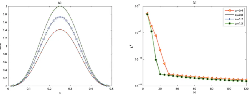
In Figure 1, we report the L∞−norm error defined as
L∞(N) = ||u−u¯||∞
||u||∞
= max
16j6N
|uj−u¯j|
|uj|
, (2.16)
whereu¯anduare the approximate and exact solutions, andN represents the computational grids number, onx∈ [0,0.5]
att = 1and initial conditionu0(x) = exp[−10x2/(1−x2)]. The reference solution is taken by evaluating the fractional diffusion equation using212Fourier modes. It is proper to say that regardless of fractional powerα, our approach (Fourier transform) is able to attain a spectral convergence up to machine precision.
Table 1.The relative error for fractional diffusion equation for various values of discretization, atD= 0.5andt= 1.
N N = 64 N = 128 N= 256 N = 512
RK4 1.1960e-06 4.9539e-06 7.5637e-06 1.5528e-05 ETDRK4 1.6391e-08 2.0899e-08 2.9017e-08 4.7984e-08
Figure 1.(a) Comparison of the numerical and analytical solutions of the fractional diffusion equation atα= 1.5, D= 0.5, obtained at instances oft= 2
(dots),t= 3(circles) andt= 4(crosses). The thick lines represent the analytical solutions. Panel (b) indicates convergence of the fractional Fourier method at instances ofαat final timet= 1.
Timing results (independent of fractional powerα) are given in Table 1 for comparison between both schemes. Indication here is that, the ETDRK4 displays a better performance when used in conjunction with the Fourier spectral method, especially whenNis large. In terms of efficiency and accuracy, Fourier methods when compared to low-order methods have proven to be advantageous relative to memory requirement, computationally efficient and fast in execution times. The result obtained in Table 1 justifies the reason for abandoning the RK4 scheme in the main computations.
3
Main model
Over the years, mathematical modelling has become an important tool in the application areas medical and life sciences to address some of the health challenging problems that are not approachable experimentally. Hepatitis B is commonly referred to as a life threatening infectious disease caused by the Hepatitis B virus (HBV) which leads to inflammation or causing serious damage to the liver. According to World Health Organization’s (WHO) 2002 data report, over 2,000 million people have been effected, more than 350 million individuals remain chronically infected and carriers of the virus. An estimated population of 4 million people are considered as acute clinical cases of the virus.
Research have shown that children and adolescents are most vulnerable to the disease than adults due to exposure which may show some clinical symptom and have a higher percentage chance of being acutely infected. Based on report, about a quarter of chronic infected individuals die of liver cancer annually. As a result, Hepatitis B is known to be one of the most common viral source of cancer in the world nowadays. Hence, HBV infection is a disease of global health and its prevalence varies from one region to the other.
A lot of researchers have worked on HBV in the past, among which are the notable papers of Medley et al. [18] where compartmentalized model was used to describe the spread of the disease. Almost a decade later, Zou et al. [52] worked on the modified version of the model [18]. They develop a model to explore the impact of vaccination and other controlling measures of HBV infection. Their model has simple dynamical behavior which has a globally asymptotically stable disease-free equilibrium when the basic reproduction numberR0 < 1, and a globally asymptotically stable endemic equilibrium whenR0>1. In the year 2014, Kimbir et al. [16] give an extension to the earlier report in [52] by including the treatment of chronically infected HBV carriers, it was also suggested in their report that the acute infected individuals are not subjected to antiviral treatment due to natural recovery. Wiah et al. employed a nonlinear extended deterministic model to address the impact of immigration on the population spread of HBV infection with acute and chronic infected carriers.
In this work, we present a deterministic model consisting of coupled nonlinear fractional partial differential equations of orderα. This new model provides an extension of the models discussed earlier by [52, 53]. The model population consists of five local kinetics broken into the susceptible individuals(U1), exposed class(U2)which are infected but yet to be infectious, acute infection individuals(U3), chronic HBV class(U4)and temporary protective immunity referred to as the recovered individuals(U5). The fractional reaction-diffusion system is given as
∂Ui
∂t −Di ∂αU
i
∂xα =Fi(Ui), i= 1, . . . ,5, t >0 (3.17)
whereu = (u1, u2, . . . , un)is a vector of concentration or density for interacting species at position xand timet, and
Fi, i = 1, . . . ,5, are the local reaction terms. The termsDi >0, i= 1, . . . ,5are the diffusion coefficients. The initial
densities are expected to be non-negative and the problem (3.17) is confined by imposing the appropriate choice of boundary conditions.
The boundary conditions are taken as zero flux
∂U1
∂x
x=0
= ∂U1
∂x
x=L
with similar relations for theUi, i = 2, . . . ,5. The initial data are taken as in equation (1.2) in the form of some small
perturbations from the uniform solution *:
U1(x,0) =Ui∗+Ui0(x), |Ui0(x)| |Ui∗| (3.19)
with analogous expressions for the remaining species. subject to the following coupled reaction kinetics F1(U1, U2, . . . , U5) = γ−ω(U3+ψU4)U1−(τ+φ)U1,
F2(U1, U2, . . . , U5) = ω(U3+ψU4)U1−(δ++τ)U2,
F3(U1, U2, . . . , U5) = δU2−[(1−ϕ)σ−τ]U3, (3.20) F4(U1, U2, . . . , U5) = (1−ϕ)σU3−(τ−β)U4,
F5(U1, U2, . . . , U5) = φU1+U2−τ U5
whereγrepresents the rate of recruitment into a susceptible individuals,ωstands for the transmission rate of disease from one infection class to another. The HBV induced rate is given byβ, whileτis the natural death rate. Parametersδ, σare the progressive rate from the exposed(U2)to acute(U3) infection individuals and acute to chronic infection class(U4) respectively. The natural recovery rate for the exposed individuals for the latent HBV is denoted by, whileψ 1is the transmission rate multiplier. Finally,φandϕare the respective vaccination success rate for the classU1and treatment success rate for(U3)infected class.
3.1
Stability analysis of the disease free equilibrium (DFE) point
In this section, we analyze the local stability of the disease-free equilibrium (DFE). It is the stability of at DFE that can guarantee a biologically meaningful results. Here we assume that the disease variablesU2=U3=U4= 0. If otherwise, the disease will persist and put the whole population of susceptible individuals into serious danger.
The basic reproduction number, commonly denoted asR0, gives the total number of secondary infections that an average infectious class will induce given that the rest of the population is susceptible. By using the notation in Pang et al. [25], we denote the emergence of new infection byF, and the transfer of individual from one class to another byV. The endemic equilibrium dynamics in the region(U1>0, U2>0, U3>0, U4>0, U5>0) = ( ˆU1,Uˆ2,Uˆ3,Uˆ4,Uˆ5), do not correspond to biologically meaningful results since it encourages the spread of HBV disease. Hence, we do not capture the endemic equilib-rium results in the analysis. For all possible parameter values, the spatially homogeneous stationary solution of model (3.17) with kinetics (3.20) has a disease free equilibrium pointEˆ = (γ/(τ+φ),0,0,0, τ φ/(τ+φ)τ), we define the reproduction number asR0= (F V−1), where
F =
0 ωτ
τ+φ ψωτ τ+φ
0 0 0
0 0 0
, V =
δ++τ 0 0
−δ τ+ (1−ϕ)σ 0 0 (ϕ−1)σ τ+β
.
After some algebraic manipulations, we obtain the average value of the expected number of secondary cases produced by a single infected individual asi
R0=
[τ+β+ (1−ϕ)ψσ]ωτ δ
(τ+β)(δ++τ)(τ+φ)((1−ϕ)σ+τ) (3.21)
Theorem 3.1. The disease free equilibrium pointEˆ= (γ/(τ+φ),0,0,0, τ φ/(τ+φ)τ)is locally asymptotically stable for the spatially homogeneous stationary solution of model (3.17) with kinetics (3.20) ifR0<1, and unstable if otherwise.
Proof. The Jacobian matrix of the spatially homogeneous stationary solution of model (3.17) with kinetics (3.20) at pointEˆ
is given by
JEˆ =
−(φ+τ) 0 − ωτ
φ+τ −
ψωτ φ+τ 0
0 −(δ++τ) ωτ
φ+τ
ψωτ
φ+τ 0
0 δ −(τ+ (1−ϕ)σ) 0 0
0 0 τ+ (1−ϕ)σ −(β+tau) 0
φ 0 0 −τ
(3.22)
From the characteristics equation of (3.22), we have two negative eigenvalues λ1 = −τ, λ2 = −(τ +φ). After substitution, we have the rest of the characteristic polynomial given as
whereAij, i, j = 1,2,3 is a 3 ×3 matrix, and Iidentity matrix. From (3.23), we obtain the characteristic equation
X(λ) =λ3−(a11a22a33)λ2+ (a11a22+a11a33+a22a33+a12a21)λ−a12a21a33−a12a22a33−a13a21a32= 0. By adopting the Routh-Hurwitz stability conditions of the linear differential equations, system (3.17) with kinetics (3.20) is stable for the disease free equilibrium pointEˆ if: (i) the rootsr0, r1, r2, r3 are positive with negative real parts, where
r3= 1, r2 =a11a22+a11a33, r1 = (a11a22+a11a33+a22a33+a12a21), r0 =a12a21a33−a12a22a33−a13a21a32(ii)
r1r2−r0a3>0. We verified from the coefficients thatr0 >0, r1>0, r2>0, r3>0andr1r2−r0a3=−R0>1which implies thatR0 < 1. Hence we complete the proof sinceR0 < 1 which shows that the disease free equilibrium point is locally asymptotically stable.
3.2
Global stability of the diseases free equilibrium point
Here, we are concerned with the global stability of DFE point. We adopt a similar technique to the proof of Theorem 3.1.
Theorem 3.2. The disease free equilibrium pointEˆ = (γ/(τ+φ),0,0,0, τ φ/(τ+φ)τ)is globally asymptotically stable for the spatially homogeneous stationary solution of model (3.17) with kinetics (3.20), ifR0<1.
Proof. LetGbe a Lyapunov function given in the form
G(Ui, t) =PU2+U3+QU4, i= 1(1)5. (3.24) On differentiating (3.24) and substitute the spatially homogeneous version of model (3.17) with kinetics (3.20) into it atEˆ, we have
G0 ≤(δ− P(ψ+δ+τ))U2+
P ωτ
φ+τ +Q(1−ϕ)σ
U3+
P ωψτ
φ+τ − Q(τ+β)
U4, (3.25)
on substituting forP = δ
τ δ andQ=
ψωτ δ
(τ δ)(τ+β)(φ+τ) in (3.25) we get
G0 ≤ (σ(1−ϕ) +τ)
[τ+β+ (1−ϕ)ψσ]ωτ δ
(τ+β)(δ++τ)(τ+φ)((1−ϕ)σ+τ)
| {z }
R0
−1
,
≤ (σ(1−ϕ) +τ)(R0−1)≤0.
It follows from the pointEˆ= (γ/(τ+φ),0,0,0, τ φ/(τ+φ)τ)thatG= 0since the derivatives ofUi= 0, i= 2,3,4. This
implies that asUi→0, i= 2,3,4, alsoU1→γ/(τ+φ)andU5→τ φ/(τ+φ)τast→ ∞. So the DFE point is globally asymptotically stable if the inequality is satisfies the conditionR0<1, but unstable ifR0>1. The proof is completed.
4
Numerical simulations
In this section, we start to simulate numerically the solution of the spatially homogeneous system (3.17) with kinetics (3.20) using the numerical techniques formulated in Section 2 above to substantiate our analytical findings.
4.1
Non-diffusive example
We consider the set of parameters
φ= 2.5, γ= 2.0, ω= 0.5, ψ = 2.5, δ= 0.5, = 1.5, ϕ= 0.75, β= 2.5 (4.26) with reasonable initial populations (millions)
U1(0) = 95.5, U2(0) = 2.0, U3(0) = 3.0, U4(0) = 1.5, U5(0) = 1.0. (4.27) For the set of ecological parameters, we realized that the conditions given in Theorems 3.1 and 3.2 for non-diffusive system are satisfied for the disease free-equilibrium state.
In Figure 2, we simulate the non-diffusive system numerically at different instances oftauto study the behaviour of the species with time (year)t= 1. It was observed only the class of individualsU1, U2, U5could actually be free of HBV as time is progressed. Clearly, those in the classesU3andU4which corresponds to the number of acute and chronic individuals will continue to live and spread the virus as years roll-by until the entire population is endermic.
Figure 2.Time series results for the spatially homogeneous version of system (3.17) with kinetics (3.20), obtained at different instants ofτand final time
t= 1. Other parameters are fixed in (4.26).
Figure 3.Time series results for the spatially homogeneous version of system (3.17) with kinetics (3.20), obtained at different instants ofand final time
[image:9.595.76.531.505.734.2]Since it is not possible to completely wipe out bothU3andU4classes in model (or in the population). Then, the question of ’what can be done?’ sets in. In the context of this paper, we came out with the opinion of varying some of the parameters, the correct choice of parameters that will put control to the spread of HBV is attained by reducing the values ofτfrom1.5
[image:10.595.75.494.154.480.2]to0.5and that ofβfrom2.5 → 0.05to enable the class of individualsU4respond to treatment over time. To checkmate the spread of HBV for the groupU3, we need to increase parameter valueδfrom1.5to10.5and above. These assertion is evident in Figure 4.
Figure 4.Behaviour of the acute and chronic individuals to treatment at instancesδand timet. Parameters are:τ= 0.5, β= 0.05att= 5andt= 10
for speciesU3andU4. Both species respond to treatment at the control parameters level with respect to time. Other parameters are fixed in (4.26).
4.2
Fractional reaction-diffusion example
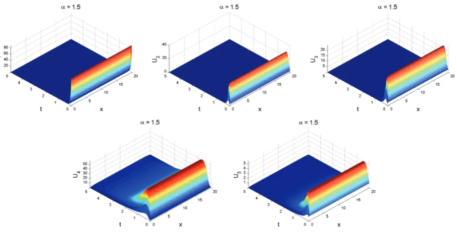
Here, we simulate the whole system in the presence of diffusion with fractional power indexα. We now illustrate through numerical experiments with Neumann boundary conditions, a multiple coexistence steady states in the fractional-in-space reaction-diffusion model (3.17) with kinetics (3.20). The boundary conditions are clamped the the extreme points of spatial domain of size[0, L], L= 20. We compute the initial conditions as:
U1=95.5*ones(N,1);U2=2*ones(N,1);U3=3*ones(N,1);U4=1.5*ones(N,1);U5=1*ones(N,1);
whereNis the number of discretisation. We fixed parameters as:
{φ = 2.5, τ = 1.5, γ= 2.0, ω= 0.5, ψ= 2.5, δ= 1.5, = 0.5,
ϕ = 0.75, β= 2.5, D1= 0.2, D2= 0.5, D3= 0.25, D4= 0.1, D5= 0.5} (4.28) to obtain the surface plots displayed in Figure 5. Obviously, the behaviour of the species correspond to those in Figures 2 and 3, though the amplitudes differ.
Figure 5.Surface plots for fractional reaction-diffusion system (3.17) with kinetics (3.20) at sub-diffusive scenario whenα= 0.5andt= 3. The dynamics obtained are similar to those presented in Figures 2 and 3. Parameters are given in (4.26).
[image:11.595.80.533.503.733.2]5
Conclusion
In this paper, a mathematical model for investigating the Hepatitis B Virus disease in fractional medium is derived. The model disease free equilibrium state is analyzed. We established via theorems that the model disease-free equilibrium is both locally and globally asymptotically stable, if the basic reproduction number is less than unity. Our aim is to examine the behaviour of diffusive fractional reaction-diffusion model in sub-diffusive and super-diffusive scenarios, derive efficient and reliable numerical techniques. By the computer experiment of the fractional reaction-diffusion system we have given enough evidence that numerical solution in the diffusive (fractional) scenario, at0< α <2is practicably the same as in the case of non-diffusive case when applied to model Hepatitis B virus system. Our findings in this work strongly recommend a combination of effective treatment and vaccination as a good control measure is important to record the success of HBV disease control. It should be noted that the methodology presented in this paper can be applied to model other physical phenomena in higher dimensions.
Competing Interests
The author declares that there is no conflict of interests regarding the publication of this paper.
Author’s Contributions
The whole work-done in this research paper is carried out by OK.
REFERENCES
[1] A.K. Alomari, M.S.M. Noorani and R. Nazar, Explicit serie solutions of some linear and nonlinear Schr´odinger equations via the homotopy analysis method, Communications in Nonlinear Science and Numerical Simulation, 14 (2009) 1196-1207. DOI:10.1016/j.cnsns.2008.01.008
[2] A. Atangana, On the stability and convergence of the time-fractional variable order telegraph equation,Journal of Computational Physics,293(2015) 104-114.
[3] E. Barkari, R. Metzler and J. Klafter, From continuous time random walks to the fractional Fokker-Planck equation, Physical Review E,61(2000) 132-138. http://dx.doi.org/10.1103/PhysRevE.61.132
[4] C. Celik and M. Duman, Crank-Nicolson method for the fractional diffusion equation with the Riesz fractional derivative,Journal of Computational Physics,231(2012) 1743-1750. http://dx.doi.org/10.1016/j.jcp.2011.11.008
[5] W. Chen, L. Ye and H. Sun, Fractional diffusion equations by Kansa method,Computers and Mathematics with Applications59
(2010) 1614-1620.
[6] S.M. Cox and P.C. Matthews, Exponential time differencing for stiff systems,Journal of Computational Physics,176(2002) 430-455.
[7] X. Li Ding and Y. Lin-Jiang, Analytical solutions for the multi-term time-space fractional advection-diffusion equations with mixed boundary conditions,Nonlinear Analysis: Real World Applications,14(2013) 1026-1033.
[8] V. Erturk, Z. Odibat and S. Momani, An approximate solution of a fractional order differential equation model of human T-cell lymphotropic virus (HTLV-I) infection of CD4 T-cells,Computers and Mathematics with Applications,62(2011) 996-1002.
[9] A.R. Haghighi, A. Dadvand and H.H. Ghejlo, Solution of the fractional diffusion equation with the Riesz fractional deriva-tive using McCormack method, Communications on Advanced Computational Science with Applications 2014 (2014) 1-11. doi:10.5899/2014/cacsa-00024
[10] M.G. Hall and T.R. Barrick, From diffusion-weighted MRI to anomalous diffusion imaging,Magnetic Resonance in Medicine,59
(2008) 447-455. http://dx.doi.org/10.1002/mrm.21453
[11] I.H. Hassan, Comparison differential transformation technique with Adomian decomposition method for linear and nonlinear initial value problems,Chaos Solitons & Fractals,36(2008) 53-65. DOI:10.1016/j.chaos.2006.06.040
[12] J.H. He, Application of homotopy perturbation method to nonlinear wave equations,Chaos Soliton & Fractals,26(2005) 695-700. http://dx.doi.org/10.1016/j.chaos.2005.03.006
[13] H. Jiang, F. Liu, I. Turner and K. Burrage, Analytical solutions for the multi-term time-space Caputo-Rieze fractional advection-diffusion equations on a finite domain, Journal of Mathematical Analysis and Applications, 389 (2012) 1117-1127. http://dx.doi.org/10.1016/j.jmaa.2011.12.055
[15] A.A. Kilbas, H.M. Srivastava and J.J. Trujillo,Theory and applications of fractional differential equations, New York: Elsevier; 2005.
[16] A.R. Kimbir, T. Aboiyar, O. Abu and E.S. Onah, Simulation of A Mathematical Model of Hepatitis B Virus Transmission Dynamics in the Presence of Vaccination and Treatment, Mathematical Theory and Modeling,4(2014) 44-59.
[17] S. Krogstad, Generalized integrating factor methods for stiff PDEs,Journal Computational Physics203(2005), 72-88.
[18] G.F. Medley, N.A. Lindop, W.J. Edmunds and D.J. Nokes, Hepatitis-B virus endemicity: heterogeneity, catastrophic dynamics and control.Nature Medicine7(2001) 619-624.
[19] M.D. Ortigueira, Riesz potential operators and inverses via fractional centred derivatives,International Journal of Mathematics and Mathematical Sciences, (2006) 1-12. http://dx.doi.org/10.1155/IJMMS/2006/48391
[20] S. Otte, S. Berg, S. Luther and U. Parlitz, Bifurcations, chaos, and sensitivity to parameter variations in the Sato cardiac cell model, Communications in Nonlinear Science and Numerical Simulation37(2016) 265-281. http://dx.doi.org/10.1016/j.cnsns.2016.01.014
[21] K.M. Owolabi and K.C. Patidar, Higher-order time-stepping methods for time-dependent reaction-diffusion equations arising in biology,Applied Mathematics and Computation240(2014), 30-50. http://dx.doi.org/10.1016/j.amc.2014.04.055
[22] K.M. Owolabi and K.C. Patidar, Existence and permanence in a diffusive KiSS model with robust numerical simulations, Interna-tional Journal of Differential Equations,2015; 2015(485860):8. doi:10.1155/2015/485860.
[23] K.M. Owolabi and K.C. Patidar, Numerical simulations of multicomponent ecological models with adaptive methods,Theoretical Biology and Medical Modelling13(2016), DOI 10.1186/s12976-016-0027-4.
[24] K.M. Owolabi and K.C. Patidar, Effect of spatial configuration of an extended nonlinear KiersteadSlobodkin reactiontransport model with adaptive numerical scheme,Springer Plus(2016)5:303. DOI 10.1186/s40064-016-1941-y
[25] J. Pang, J. Cui and X. Zhou, Dynamical behavior of a hepatitis B virus transmission model with vaccination,Journal of Theoretical Biology,265(2010) 572-578.
[26] H.K. Pang and H.W. Sun, Multigrid method for fractional diffusion, Journal of Computational Physics,231(2012) 693-703.
[27] E. Pindza, K.M. Owolabi, Fourier spectral method for higher order space fractional reaction-diffusion equations,Communications in Nonlinear Science and Numerical Simulation40(2016) 112-128. doi: 10.1016/j.cnsns.2016.04.020
[28] I. Podlubny,Fractional differential equations, Academic Press, San Diego, 1999.
[29] I. Podlubny, A. Chechkin, T. Skovranek, Y.Q. Chen and B.B. Jara, Matrix approach to discrete fractional calculus II: Partial fractional differential equations,Journal of Computational Physics,228(2009) 3137-3153.
[30] A.D. Polyanin and V.F. Zaitsev,Handbook of Nonlinear Partial Differential Equations, Chapman & Hall/CRC, Boca Raton, FL, 2004.
[31] S.S. Ray, Analytical solution for the space fractional diffusion equation by two-step Adomian Decomposition Method, Communica-tions in Nonlinear Science and Numerical simulation,14(2009) 1295-1306.
[32] A. Saadatmandi and M. Dehghan, A tau approach for solution of the space fractional diffusion equation,Computers & Mathematics with Applications,62(2011) 1135-1142. http://dx.doi.org/10.1016/j.camwa.2011.04.014
[33] S.G. Samko, A.A. Kilbas and O.I. Marichev,Fractional Integrals and Derivatives: Theory and Applications, Gordon and Breach, Amsterdam, 1993.
[34] E. Sausa, Finite difference approximations for a fractional advection diffusion problem,Journal of Computational Physics, 228
(2009) 4038-4054.
[35] R.K. Saxena, A.M. Mathai and H.J. Haubold, Fractional reaction-diffusion equations,Astrophysics and Space Science,305(2006) 289-296.
[36] L. Su, W. Wang and Q. Xu, Finite difference methods for fractional dispersion equations,Applied Mathematics and Computation,
216(2010) 3329-3334. http://dx.doi.org/10.1016/j.amc.2010.04.060
[37] Z. Tomovski, T. Sandev, R. Metzler and J. Dubbeldam, Generalized space-time fractional diffusion equation with composite fractional time derivative, Physica A: Statistical Mechanics and its Applications,391(2012) 2527-2542.
[38] M.A. Jafari and A. Aminataei , An algorithm for solving multi-term diffusion-wave equations of fractional order,Computers and Mathematics with Applications,62(2011) 1091-1097.
[39] S.K. Vanani and A. Aminataei, Tau approximate solution of fractional partial differential equations,Computers and Mathematics with Applications,62(2011) 1075-1083.
[40] S.K. Vanani and A. Aminataei, A numerical algorithm for the space and time fractional Fokker-Planck equation,International Journal of Numerical Methods for Heat and Fluid Flow,22(2012) 1037-1052.
[42] J.R. Wang and Y. Zhou, A class of fractional evolution equations and optimal controls,Nonlinear Analysis: Real World Applications
12(2011) 262-272. http://dx.doi.org/10.1016/j.nonrwa.2010.06.013
[43] J.R. Wang, Y. Zhou and W. Wei, Fractional Schrodinger equations with potential and optimal controls,Nonlinear Analysis: Real World Applications13, (2012) 2755-2766. http://dx.doi.org/10.1016/j.nonrwa.2012.04.004
[44] H. Wang and N. Du, A super fast-preconditioned iterative method for steady-state space fractional diffusion equations,Journal of Computational Physics240(2013) 49-57.
[45] Q. Yang, F. Liu, I. Turner, Numerical methods for fractional partial differential equations with Riesz space fractional derivatives, Applied Mathematical Modeling, 34 (2010) 200-218. (doi:10.1016/j.apm.2009.04.006)
[46] A. Yildirim and S.A. Sezer, Analytical solution of linear and nonlinear space-time fractional reaction-diffusion equations, Interna-tional Journal of Chemical Reactor Engineering,8(2010) 1-21.
[47] S.B. Yuste, L. Acedo and K. Lindenberg, Reaction front in an A+BC reaction-subdiffusion process,Physical Review E,69(2004) 036126.
[48] F. Zeng, C. Li, F. Liu, and I. Turner, Numerical algorithms for time-fractional subdiffusion equation with second-order accuracy, SIAM Journal on Scientific Computing,37(2015) A55-A78.
[49] F. Zeng, F. Liu, C. Li, K. Burrage, I. Turner and V. Anh, A Crank-Nicolson ADI spectral method for a two-dimensional riesz space fractional nonlinear reaction-diffusion equation,SIAM Journal on Numerical Analysis,52(2014) 2599-2622.
[50] M. Zheng, F. Liu, I. Turner and V. Anh, A Novel High Order Space-Time Spectral Method for the Time Fractional Fokker-Planck Equation,SIAM Journal on Scientific Computing,37(2015), A701-A724.
[51] Y. Zhou,Basic Theory of Fractional Differential Equations, World Scientific, New Jersey, 2014.
[52] L. Zou, W. Zhang and S. Ruan, Modelling the transmission dynamics and control of hepatitis B virus in China,Journal of Theoretical Biology262(2010) 330-338.
[53] L. Zou, S. Ruan and W. Zhang, On the sexual transmission dynamics of hepatitis B virus in China,Journal of Theoretical Biology