Job Scheduling in the Grid Computing using Criteria
Latha C A,
Ph.D Prof., Dept. of CS & E D B I T, Bangalore-74ABSTRACT
Clusters of computers have emerged as mainstream parallel and distributed platforms for high performance, high throughput, and high availability computing. To enable effective load balancing in distributed systems, numerous schedulers have been designed. Migration of the job from an overloaded node to the idle node, involves matching the possessions of the idle computer with the job requirements. Both code and data are to be transferred to the idle node from overloaded node. The job is executed at the idle node. The results are transferred back to the host node. These consume a lot of bandwidth, processor time, and memory. A good selection of job results in less execution time, efficient usage of resources and overall increase in the throughput of the system with the minimum cost. The selection of the job and its subsequent execution is an interesting area of research. The proposed criteria based method assigns a weight for each criterion of each job of several predefined criteria. Then the total weights of all the jobs are found out. The job with the highest weight will be considered for submission.
Key words
Distributed system, load balance, Idle, overloaded, criteria, weight,
1.
INTRODUCTION
When jobs are submitted for execution in a parallel system, they are typically first organized in a job queue. From there, they are selected for execution by the scheduler. Early scheduling strategies for distributed systems just used a space-sharing approach, wherein jobs can run side by side on different nodes of the machine at the same time, but each node is exclusively assigned to a job. When there are not enough nodes, the jobs in the queue simply wait. Space sharing in isolation can result in poor utilization, as nodes remain empty despite a queue of waiting jobs. Furthermore, the wait and response times for jobs with an exclusively space-sharing strategy are relatively high.
Many applications running on grids take large amount of input data and perform complex computation to produce useful information. Grid systems are often built across wide area network. They often consist of many nodes, distributed geographically. The cost to transfer input data thus plays an important role on the overall efficiency of the application. Due to the heterogeneous nature of the wide area network, the computing sites in grid system often differ from each other on their computing and communication capabilities. After finding an idle node, a job has to be selected from the queue of over loaded computers in the network. This selected job has to be migrated and processed at the idle system.
When jobs are submitted for execution in a parallel system, they are typically first organized in a job queue. From there,
they are selected for execution by the scheduler. Once the idle computer is identified, it is the function of the scheduler to allocate a best suitable job from the ready queue of the overloaded computer and submit it to the idle computer. As the distributed system is heterogeneous, the idle system’s resources and features should meet the requirements of the selected job from overload om ed node.
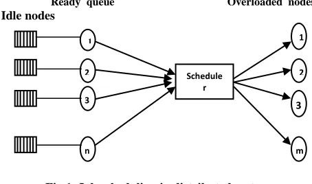
The whole concept is pictorially shown in Figure 1. Each computer has a job queue. On every node, a system task regularly computes the workload on the node and stores the information in appropriate data structures. This task runs as a periodic system task. The scheduler will collect information from all these system tasks and take a decision as to which job from which overloaded computer would be mapped to suitable available idle node. As the distributed system is heterogeneous, the idle system’s resources and features should meet the requirements of the job at overloaded computer.
Ready queue Overloaded nodes
[image:1.612.329.556.357.491.2]Idle nodes
Fig 1. Job scheduling in distributed system
2.
PROPOSED CRITERIA BASED
METHOD
This work is based on the assumption that, in the distributed system, the idle node and an overloaded node are already identified for load balancing. First, idle computer’s specifications are matched with that of overloaded node’s specifications with reference to different attributes, example, operating system, speed, and the resources required etc. Alternately, the job requirements can be checked with the specification of the idle computer. There is a tradeoff between these two schemes. If it is desired to reduce the processing time for selection, then latter match becomes more demanding in terms of computations. All the jobs in the queue need to be checked. However, such a check becomes a foolproof approach for determination of the job to be selected. Next question is who has to do this matching and checking process. Overloaded node is already busy with the jobs. Hence, it is proposed the idle node to perform this matching and checking process. The overhead required for this selection may be very
1
2
3
n
Schedule r
1
2
3
6 nominal. The following section shows how the weights are
assigned for each job and the winning factor is calculated based on which the scheduling is accomplished.
2.1. Job selection criteria
Consider the jobs at the ready queue of the overloaded node. Each job is given a weight for its value of each criterion considered, as demonstrated in the following tables. The table in each criterion discussion shows, how the jobs are assigned weights corresponding to their criterion values. The tables are discussed for an example of a system with 10 jobs J1 to J10.
First criterion considered is the real-time or nonreal-time job.
Real-time jobs are assigned a weight of one and nonreal-time jobs are assigned weight of zero.
[image:2.612.74.310.328.410.2]Real-time jobs should be given highest importance which needs to be scheduled at the earliest possible. Hence, assign the real-time job indicated by R a highest weight of one and nonreal-time job indicated by N a weight of zero. A sample of 10 jobs with different status of real time processing and the corresponding weights assigned is shown in Table 1.
Table 1: Weight assignment for real time processes
Job J1 J2 J3 J4 J5 J6 J7 J8 J9 J10
Real-time or Non real-time
R R N N R N N R R N
Weight assigned 1 1 0 0 1 0 0 1 1 0
Waiting time the process has spent already.
More the waiting time the process has spent, Higher is the weight assigned.
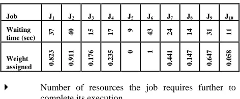
This is to ensure that the processes, which have been waiting for a long time at the overloaded node, are to be processed at the earliest. Hence, to enable the job to be submitted at the idle node earliest possible, a higher weight close to one is assigned. If the job has arrived just then, then it can afford to wait for some time more. Hence, to delay its submission at the idle node, a lower weight towards zero is assigned. Hence, the weight is assumed to be continuous in the range of zero to one. A sample of 10 jobs with different values for time spent in waiting and the corresponding weights assigned is shown in Table 2.
Table 2: Weight assignment for waiting time
Job J1 J2 J3 J4 J5 J6 J7 J8 J9 J10
Waiting
time (sec) 37 40 15 17
9 43 24 14 31 11
Weight assigned 0.
823
0.
911
0.
176
0.
235
0 1
0.
441
0.
147
0.
647
0.
058
Number of resources the job requires further to complete its execution
More the number of resources the job requires, lesser is the weight assigned.
[image:2.612.325.564.338.458.2]As we are looking for job to be migrated to achieve load balancing, lesser the message length and information to be transferred better is the performance. Therefore, more the resources, especially logical resources, larger will be message and the information to be transferred along with the code. To acquire the ownership of all the remote or local resources also takes time. Instead, if the submission is delayed, there are chances of it being executed locally once the host node becomes moderately loaded. In addition, if the job is scheduled and all those resources are allotted to this job, then many other jobs requiring those resources would be delayed. This decreases the overall throughput of the system. Hence, to delay the submission, the weight is set to a lower value towards zero. However, if the number of resources is less, then it is easier for the remote idle processor to acquire the ownership of the minimum number of resources. Hence, to enable such processes to be migrated and submitted at the idle node at the earliest possible, the weight is set to a higher value towards one. Hence, the weight is assumed to be continuous in the range of zero and one. A sample of 10 jobs with different resources requirement for processing the jobs and the corresponding weights assigned is shown in Table 3.
Table 3: Weight assignment for resources requirement
Job
J1 J2 J3 J4 J5 J6 J7 J8 J9 J10
No. of resourc es the job requires
25 60 49 31 42 45 60 31 60 55
Weight assigne d
1.
0
0.
0
0.
314
0.
829
0.
514
0.
429 0.0
0.
829 0.0
0.
143
Number of resources already the process has
More the number of resources the process has, higher is the weight assigned.
[image:2.612.74.310.581.679.2]Table 4: Weight assignment for resources possession
Processor time already consumed by the process
More the processor time consumed, higher the weight assigned.
This is with the expectation that the process which has already consumed majority of its required processor time, given another short span of processor time, processor will complete the execution of the job and release the resources acquired to the resources’ pool. Hence, the process that has consumed more processor time will have to be completed earlier. Therefore, assign a higher weight towards one. On the contrary, lesser the processor time already consumed, it can afford a delay in submission. Hence, assign a lesser weight towards zero. Hence, the weight is assumed to be continuous in the range of zero and one. A sample of 10 jobs with different status of processor time spent and the corresponding weights assigned is shown in Table 5.
Table 5: Weight assignment for processor time spent
Job J1 J2 J3 J4 J5 J6 J7 J8 J9 J10
Processor time the job has spent (sec)
9 8 5 8 12 12 15 14 11 3
Weight assigned
0.
500
0.
417
0.
167
0.
417
0.
750
0.
750 1.
0
0.
917
0.
667
0
Estimated processor time required to complete the execution of the process.
More the processor time required to complete its execution, lesser is the weight assigned.
If the process requires comparatively more processor time to complete its execution and if scheduled at a remote idle computer, then it causes many problems. Some of them to mention, until the process is completed the other processes should wait for a long time, which decreases overall throughput of the system. If it takes a longer processor time at the remote idle machine, then a local job arriving at the idle machine will have to wait until its completion, which violates the requirement of giving higher priority to the local jobs. Another problem, if the process takes a longer execution time, then usually it implies the job is very big. Transferring such a huge job from the overloaded node to the idle node induces a huge overhead and propagation delay. Hence, scheduling such jobs at the idle nodes should be postponed as later as possible. Therefore, assign a lower weight towards zero. On the contrary, those jobs requiring lesser time to complete their execution can be transferred at a relatively lower cost. Hence, they can be scheduled immediately. Therefore, they are
[image:3.612.328.561.147.255.2]assigned relatively higher weights towards one. Hence, the weight is assumed to be continuous in the range of zero and one. A sample of 10 jobs with different status of processor time required to complete the execution and the corresponding weights assigned is shown in Table 6.
Table 6: Weight assignment for processor time required
Job J1 J2 J3 J4 J5 J6 J7 J8 J9 J10
Processo r time required (seconds)
10 9 5 1 6 12 8 9 11 6
Weight
assigned 0.182 0.273 0.636 1.000 5450. 0.000 0.364 0.273 0.091 0.545
Number of children or dependent jobs
More the number of dependent jobs, higher the weight assigned.
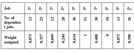
If a process has many children or dependent processes, delaying that job leads to automatic delaying of all those dependent processes. To avoid that, such jobs should be submitted at the earliest. Therefore, those jobs are assigned a higher weight towards one. Jobs with lesser number of children or dependent jobs can afford the delay with comparatively lesser cost. Accordingly, they are assigned relatively lower weight towards zero. Hence, the weight is assumed to be continuous in the range of zero and one. A sample of 10 jobs with different values of number of dependent jobs and the corresponding weights assigned is shown in Table 7.
Table 7: Weight assignment for dependent jobs
Job J1 J2 J3 J4 J5 J6 J7 J8 J9 J10
No. of dependen t jobs
13 23 12 20 36 51 30 10 13 26
Weight
assigned 0.073 0.317 0.049 0.244 0.634
1
0.
488
0
0.
073
0.
390
Priority of the job
Higher the priority of the job, higher the weight assigned.
Priorities can be set based on various parameters. Higher the priority of the job, earlier it should be executed. Hence, higher weight is assigned with value towards one. Lower the priority, longer it can afford to wait. Accordingly, they are assigned a lower weight with value towards zero. Hence, the weight is assumed to be continuous in the range of zero and one. A sample of 10 jobs with different priorities and the corresponding weights assigned is shown in Table 8.
Job J1 J2 J3 J4 J5 J6 J7 J8 J9 J10
No. of resources the job has
32 53 36 66 34 70 32 66 21 52
Weight
assigned 0.224 0.653 0.306 0.918 0.265
1
0.
224
0.
918
0
0.
632
[image:3.612.73.311.372.500.2] [image:3.612.328.562.426.521.2]8
Table 8: Weight assignment for jobs’ priority
Job J1 J2 J3 J4 J5 J6 J7 J8 J9 J10
Priority of the job
7
19 8 1 8 13 7 11 19 2
Weight assigne
d 0.333
1.
0
0.
389 0.
0
0.
389
0.
667
0.
333
0.
556 1.
0
0.
056
Size of the job
Larger the job, lesser the weight assigned.
[image:4.612.70.315.366.461.2]Transferring a huge job from the overloaded node to the idle node induces overhead of routing, error checking and retransmissions, packeting and assembling and the propagation delay. Hence scheduling such jobs at the idle nodes should be postponed as later as possible. Accordingly, assign a lower weight towards zero. On the contrary, those smaller jobs can be transferred at a relatively lower cost. Hence, they can be scheduled immediately. Therefore, such jobs are assigned relatively higher weights towards one. Hence, the weight is assumed to be continuous in the range of zero and one. A sample of 10 jobs of various sizes and the corresponding weights assigned is shown in Table 9.
Table 9: Weight assignment for size of the jobs
Having set the weights for all jobs at the overloaded computer, considering all the criteria, the winner factor, ‘µ’ is calculated as,
m-1
µi = ∑Wij where i is the process-id and j is the
j=0 criterion
That is, µi is the total weight assigned to process i,
for all criteria j = 0 to m-1.
The procedure is repeated for all n jobs in the queue of the considered overloaded computer. Now the jobs are scheduled by selecting a job with the highest weight. The job p will be scheduled before job q, if and only if µp > µq for all p and q. If
there are two or more jobs with the same weights, then the resources needed for each job and the available resources is considered. One job, which can be given all the required resources at that instant, so that waiting time of that job (in turn of all other jobs) will be reduced, can be selected. As can be expected, this increases the throughput of the system.
For all the criteria of each job, weight is set in the range of zero and one, proportionate to value of the criterion. The scheduler, after collecting the information about all the jobs at the overloaded computer, finds the largest of all the values for a criterion. It then sets the weight to highest as normalized one. Similarly, the smallest of all the values for a criterion will be set to the least normalized value as zero. The remaining values are assigned proportionately ranging between zero and one.
2.2 Implementation
Distributed system is known to be highly dynamic. Hence, the algorithm is implemented on a heterogeneous environment. The heterogeneous environment is created by making both jobs and nodes highly dynamically heterogeneous. The attributes such as, operating system, number of resources required, number of resources the processor already has, the processor time required to complete the execution etc. are randomly generated. There are 25 nodes and 150 jobs submitted. The nodes are set to various configurations randomly. The jobs are assigned different values for all the criteria considered in the proposed method. The Table 10 shows the values of all those criteria and the corresponding normalized weight assigned to that criteria in the next column. The last column gives the winner factor based on which the scheduling takes place. The first and the third columns give the source and the destination machine ids. The different values for source and destination ids imply the job being migrated and executed remotely, showing an attempt of load balancing. The same values for source and destination ids imply local execution.
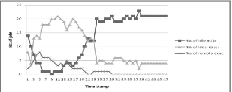
Figure 2 shows the status of execution as time elapses. It is captured for a span of first 47 timestamps. Each timestamp indicates one simulation time. It can be seen that in the beginning the number of idle machines goes on getting reduced. To be precise, until timestamp 9, the number of idle machines decreases demonstrating load-balancing activity taking place. After some time, the number of idle machines is increased. This is because, the overloaded machines have become moderately loaded. The case may also be that the jobs from overloaded machines, which can be executed at any idle machine, are exhausted. That is, the remaining jobs require the host machines only for many reasons. Hence, gradually remote execution reaches almost zero.
Fig 2 Execution statuses of idle and overloaded nodes
Job J1 J2 J3 J4 J5 J6 J7 J8 J9 J10
Size of
the job (MI)
199 192 25
7
124 156 38 71 18 128
Weight assigne d
0.
0
0.
036
0.
906 1.
0
0.
391
0.
224
0.
839
0.
667
0.
943
0.
[image:4.612.330.559.539.630.2]Fig 3 Performance of with and without the proposed algorithm
Figure 3 shows a comparative analysis of the distributed system with and without the proposed algorithm. The triangle bits line shows the number of idle nodes with the algorithm and square bits line shows the number of idle nodes without the algorithm. It clearly shows the number of idle machines is reduced by 22 with the usage of algorithm. This accounts to 14% of better processor utilization.
3.
CONCLUSION
The research work focuses on scheduling the job of an overloaded node to be executed at the idle computer. In this approach, weights are assigned to each of the job for each of the criteria. Having set the weights, the winner factor, the summation of all the weights of all the criteria is calculated. The procedure is repeated for all the jobs in the queue of the considered overloaded computer. The jobs are scheduled one by one by selecting the jobs with the highest weight. The whole idea is experimented considering a complete dynamic scenario of 25 nodes and 150 jobs. The experiment is repeated for both homogeneous and heterogeneous with respect to both jobs and nodes. In the above case considered it shows 14% better processor utilization. The results were very encouraging evading most of the drawbacks of state-of-the-art methods.
4.
REFERENCES
[1] J Bustos, et. al. 2008, “Load Information Sharing Polices in communication Intensive Parallel Application”, From Grids to Service and Pervasive Computing, pp.111-121. [2] Helen D. Karatza, Ralph C. Hilzer 2003, “Parallel job
scheduling in homogeneous distributed systems”, The Society for modeling and Simulation International. Simulation, Vol. 79, No. 5–6, May–June.
[3] Karatza H. D, Hilzer R. C. 2003, “Performance analysis of parallel job scheduling in distributed systems”. 36th
Annual Simulation Symposium, Mar-Apr, Orland, pp. 109-116.
[4] Karatza H. D. 2000, “A comparative analysis of scheduling policies in a distributed system using simulation”, International Journal of Simulation Systems, Science &Technology, pp. 12-20.
[5] Karatza, H.D. 2000, “Scheduling Strategies for Multitasking in a Distributed System”. The 33rd Annual. Simulation Symposium, IEEE Computer system. Apr, Washington, DC, pp. 83-90.
[6] Koip P. 2005, “Parallel Algorithms for Combinatorial Search Problems”, University of Massachusetts,
[7] Legrand, H. B. Newman 2000, “A self-organizing neural network for job scheduling in distributed systems”, Contribution to ACAT.
[8] Luling R, Monien. B 1993. “A Dynamic Distributed Load Balancing Algorithm with Provable Good Performance”, 5th ACM Symposium on Parallel Algorithms and Architectures, pp.164-173.
[9] Renato P. et. al. 2007, “A complex network-based approach for job scheduling in grid environments”, HPCC 2007, lncs 4782, pp. 204–215.
[10]Veeravalli, B. Wong Han Min 2004, “Scheduling divisible loads on heterogeneous linear daisy chain networks with arbitrary processor release time”, Vol. 15, No. 3, March, pp. 273 – 288.
[11]Zhang Y, A. Sivasubramaniam 2001, “Scheduling best-effort and real-time pipelined applications on timeshared clusters”, 13th Annual ACM Symposium on Parallel
Algorithms and Architectures, July 4-6, Crete Island, Greece, pp. 209-219.
[12]P. Agrawal, D. Kifer, and C. Olston 2008. “Scheduling Shared Scans of Large Data Files”. In Proc. VLDB, pages 958–969.
[13]J. Dean and S. Ghemawat 2008. Mapreduce: simplified data processing on large clusters. Communications of the ACM, 51(1):107–113.
[14]D. Thain, T. Tannenbaum, and M. Livny 2005. “Distributed Computing in Practice: The Condor Experience. Concurrency and Computation: Practice and Experience”, 17(2):323–356, February.
[15]M. Zaharia, D. Borthakur, J. S. Sarma, K. Elmeleegy, S. Shenker, and I. Stoica 2009. “Job Scheduling for
Multi-User MapReduce Clusters”. Technical Report
UCB/EECS-2009-55, University of California at Berkeley, April.
[16]Gulati, I. Ahmad, and C. A. Waldspurger 2009. “PARDA: Proportional Allocation of Resources for Distributed Storage Access”. In Proceedings of the Seventh USENIX Conference on File and Storage Technologies (FAST’09), pages 85–98, February.