Slop based Partitioning for Vertical Fragmentation in Distributed Database System

(1)

Slop based Partitioning for Vertical Fragmentation in

Distributed Database System

Ashish Ranjan Mishra

Department of Computer Science and Engineering Kamla Nehru Institute of Technology Sultanpur-228118, Uttar Pradesh, India

Neelendra Badal

Department of Computer Science and Engineering Kamla Nehru Institute of Technology Sultanpur-228118, Uttar Pradesh, India

ABSTRACT

A Vertical Partitioning is the process of dividing the attributes of a relation. Further, a good Vertical Partitioning puts frequently accessed attributes of the relation together in a fragment. Various researchers have proposed different algorithms for Vertical Partitioning. Still, there is a scope of improvement in previous algorithms for Vertical Partitioning. In this paper a new algorithm is proposed for Vertical Partitioning in Distributed Database System. The proposed algorithm is named as Slop Based Partitioning Algorithm (SBPA). This algorithm utilizes the Clustered Affinity Matrix (CAM), which is calculated from Attribute Usage Matrix (AUM) and Frequency Matrix (FM).

Keywords

Vertical Partitioning, Clustered Affinity Matrix, Attribute Usage Matrix, Frequency Matrix, Distributed Database System, Slop Based Partitioning Algorithm.

1. INTRODUCTION

In a Distributed Database System, the fragments of the relation are scattered over the collection of independent sites. In the Distributed Database System it may be possible that queries may not retrieve the result from the local site. It is required to communicate to the other sites to retrieve the result. Frequent communication to the other sites may result in bad Query-Response-Time (QRT). Vertical Partitioning of the relation into fragments plays a crucial role in improving the QRT. A good method for Vertical Partitioning can enhance the QRT by dividing a complex large relation into the small fragments. The most frequently accessed fragment is stored in the main memory. It causes the reduced page access from the secondary memory. In Distributed Database System a query can also divided into sub-queries that operates on different fragments. The execution of the sub-queries is performed concurrently on different fragments.

There are two partitioning approaches for a relation. First approach is Horizontal Partitioning and second is Vertical Partitioning. Horizontal Partitioning partitions the relation in the smaller relations on the basis of rows. Each smaller relation contains the same number of columns, but fewer rows. Vertical Partitioning is process of dividing the table on the basis of different columns. Vertical Partitioning divides a relation into multiple relations that contain fewer columns. A query does not require the entire attributes of a relation at the same time. Only few attributes of the relation is needed by queries. So the Vertical Partitioning is more effective in improving the QRT rather than Horizontal Partitioning. In this paper a new Vertical Partitioning algorithm SBPA is proposed for vertical partitioning.

The input parameter for this SBPA is Clustered Affinity Matrix which is calculated from Attribute Usage Matrix (AUM) and Frequency Matrix (FM). After calculating Clustered Affinity Matrix (CAM), the fragments of the relation are created from SBPA using CAM. SBPA fragments the attributes of relation using CAM where the slop diminishes very rapidly.

The rest of this paper is organized as follows. Previous work on Vertical Partitioning has been critically reviewed in section 2. In section 3 technique used in SBPA for Vertical Partitioning is described. Section 4 and section 5 describe an experimental set and experimental result respectively on the proposed Vertical Partitioning algorithm. The conclusion and future scope is described in section 6.

2. LITRETURE REVIEW

From the early of the 1970s, minimization of the disk I/O is an important topic. From that time, algorithms have been developed to reduce the I/O by making the cluster of the complex relation. This results in reduced the page access from the secondary memory.

In 1972, the first algorithm for clustering was developed by McCormick et.al. in [4] with the name of Bond Energy Algorithm (BEA). The purpose of this algorithm is to identify the cluster in the complex relation. The limitation of this algorithm is that it is hard to implement without human’s interpretation. Sometimes blocks may have overlaps and some elements do not belong to any block. So the clustering is not efficient as the user except.

In 1984, after the BEA, a new algorithm was proposed by Navathe et.al. in [5].This clustering algorithm considered the frequency of queries first time and reflects the frequency in the attribute affinity matrix on which clustering was performed. The complexity of this algorithm is O(n2) time where n is the number of times the partitioning is repeated. The complexity can be increased if overlapping is allowing. The Optimal Binary Vertical Partitioning algorithm [7] was proposed by Wesley W. Chu et.al. . It uses the branch and bound technique [3] to make a binary tree whose nodes represent the query. This algorithm reduces time complexity compared to the Navathe et.al. in [6] but it does not consider the impact of query frequency, and also its run time still grows exponentially with the number of queries.

(2)

19 queries but are not accessed together in frequent queries may

be put in the same fragment.

Eltayeb’s Optimized Scheme for Vertical Partitioning [1] algorithm is also based on the Attribute Affinity Matrix [5]. This algorithm starts with a vertex V that satisfies the minimum degree of reflexivity and then finds a vertex with the maximum degree of symmetry among V’s neighbours. Once the neighbour is found both the vertex are grouped together and put in a subset. V’s neighbour becomes the new V. The process continues to find neighbours of the most recent V recursively until a cycle is formed or no vertex is left. The next step is to compute the hit ratio of partition. If the partition hit ratio is less than predefined threshold then Find the attribute with the minimum hit to miss ratio and move it to a different subset. The limitation of this algorithm is as the above graph based vertical partitioning algorithm that infrequent queries are treated the same as frequent queries.

3. DESCRIPTION OF SLOP BASED

PARTITIONING PROCEDURE

In this section SBPA, used for Vertical Partitioning of relation, is discussed in detail. Firstly using the AUM and FM, Clustered Affinity Matrix (CAM) is calculated. After calculation of CAM, SBPA is used to make the fragments of the relation.

3.1 Attribute Usage Matrix

The Attribute Usage Matrix is used to show the attributes of relation used by a query. For each query QI and each attribute

AJ, an Attribute Usage Value 0 or 1 is associated in AUM.

The associated value is 1 if the attribute AJ is used by query

QI otherwise the value associated is 0.

J I

1 if Attribute A is used by Query Q ( , )

0 otherwise

I J

USE Q A   _

 

(1)

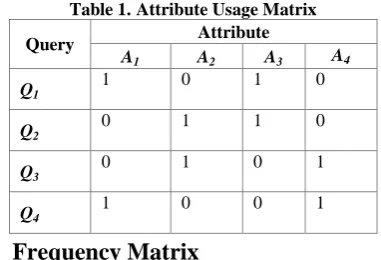
[image:2.595.354.505.71.148.2]

Each row of AUM refers the attributes used by the corresponding query. The “1” entry in a column indicates that the query “uses” the corresponding attribute. Table 1. is an example of Attribute Usage Matrix in this paper.

Table 1. Attribute Usage Matrix

Query Attribute

A1 A2 A3 A4

Q1

1 0 1 0

Q2

0 1 1 0

Q3

0 1 0 1

Q4

1 0 0 1

3.2 Frequency Matrix

The frequency matrix represents the number of time a query is fired from one or more sites. Table 2. is an example of the Frequency Matrix used in this paper.

Table 2. Frequency Matrix

Query

Site

S1 S2 S3

Q1

10 12 15

Q2

7 0 0

Query

Site

S1 S2 S3

Q3

30 25 20

Q4

5 0 0

3.3 Attribute Affinity Matrix

Attribute affinity value measures the strength of an imaginary bond between the two attributes. It is predicated on the fact that attributes are used together by the query. Attribut affinity value represents the number of times two attributes are accessed together at all sites.

Attribute affinity value between two attributes AI and AJ of a

relation R[A1,A2…AN]with respect to the set of queries

Q={Q1, Q2…QQ}is defined as follows.

Attribute affnity value between AI and AJ is represented as aff

(AI, AJ).



I J



all queries that access A and A

Aff A , A

Query access

I J

 

(2)

Where

Query access= ∑ for all sites access frequency of a query

Query access (Q1) = 37

aff (A1,A3) =∑Q1 query access=37

[image:2.595.334.523.469.585.2]

In the same way the whole Attribute affinity value is calculated.

Table 3. Attribute Affinity Matrix

Attribute Attribute

A1 A2 A3 A4

A1

42 0 37 5

A2

0 82 7 75

A3

37 7 44 0

A4

5 75 0 80

3.4 Clustered Affinity Matrix

For the fragmentation of attributes in a relation, firstly attributes must be clustered. Clustering problem is widely researched in databases, data mining and statistics communities [8], [9], [10], [11], [12], [13]. Hoffer and Severance in [2] has suggested that the Bond Energy Algorithm (BEA) should be used for this purpose. The Bond Energy Algorithm takes Attribute Affinity Matrix as input, changes the order of its rows and columns, and produces a Clustered Affinity Matrix (CAM). Bond Energy Algorithm makes the cluster of those attributes which have high Attribute affinity value.

[image:2.595.70.261.502.632.2]

(3)

 Initialization: In the initialization step, first two columns of the AAM are placed directly to the respective columns in the Clustered Affinity Matrix.

 Iteration: After the initialization step, the remaining attributes (N-I) are picked one by one and try to place them in remaining positions (I+1) Clustered Affinity Matrix. The placement is done on the basis of greatest contribution to the Global Affinity Measure. This process is continued until no more columns attribute remains to be placed.

 Row ordering: Once the placement of attribute in column is determined, the placement of row attributes should be also changing so that their relative positions match the relative positions of the columns attribute.

BEA algorithm is used to get the position of attribute in CAM. Attribute is placed to the position where contribution of placing the attribute is highest.

3.4.1 Placement of attributes in CAM

Placement of A1 and A2:

In the initialization step first and second columns of AAM is placed to the first and second column of CAM respectively. Attribute A1 is placed at position 1 in CAM: [A1]

Attribute A2 is placed at position 2 in CAM: [A1, A2]

Placement of A3:

Contribution of attribute A3 at position 1 in CAM= 6364

Contribution of attribute A3 at position 2 in CAM = 6860

Attribute A3 is placed at position 2 in CAM: [A1, A3, A2]

Placement of A4:

Contribution of attribute A4 at position 2 in CAM = - 3724

Contribution of attribute A4 at position 4 in CAM =24300

Attribute A4 is placed at position 4 in CAM: [A1, A3, A2, A4]

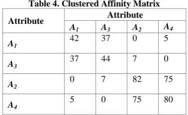
Hence in Clustered Affinity Matrix, the order of placing the attributes in rows and columns are given below:

[image:3.595.310.541.107.397.2]

[A1, A3, A2, A4]

Table 4. Clustered Affinity Matrix

Attribute Attribute

A1 A3 A2 A4

A1

42 37 0 5

A3

37 44 7 0

A2

0 7 82 75

A4

5 0 75 80

3.5 Slop Based Partitioning Algorithm

The objective of Slop Based Partitioning Algorithm is to find a set of attributes that are frequently accessed by distinct set of queries. Using the Slop Based Partitioning Algorithm, the user makes the fragments of a relation on the basis CAM, which is calculated by AUM and FM. The first row of CAM is taken for fragmenting the clusters from a relation. The point between the neighbour attributes of the CAM is considered as Split-point if slop diminishes between these attributes very rapidly. The pseudo code for the SBPA is given below: Algorithm: SBPA

Input: CAM: Clustered affinity matrix Output: F: set of two fragments Begin

{Initialization of the variables}

X [1, 1…..N]; //used to store the value from 1 to N of loop in corresponding index Y [1, 1…..N]; // used to store the value of slop Smallest=0; // used to store the smallest slop value

Split-point=0; // used to store the point from where to fragment the table {Determine the Split-point}

For i =1 to n do If (i==1) then

Y [1, i] =CAM (1, i); Else

Y [1, i] =CAM (1, i)-CAM (1, i-1); End-If

X [1, i] =i; End-For Plot (X, Y); Smallest=Y [1, 1]; Split-point=1;

For i=2 to n

If (Smallest< Y [1, i] then

Split-point is recorded as X [1, i] Smallest=Y [1, i]

End-If End-For End-Begin

This above SBPA is divided into three steps

 Initialization: In this step the user initializes the variables and array required by algorithm.

[image:3.595.72.261.508.624.2]

 Processing: In the processing step, first row of CAM is taken for fragmenting the clusters from a relation. The user takes the difference of CAM (1, i) and CAM (1, i-1) and store it at Y [1, i].

Table 5. First Row of Clustered Affinity Matrix

Attribute

A1 A3 A2 A4

A1

42 37 0 5

 Comparison: In the last step the user finds the smallest value of Y [1, i] which represents the rapid diminishing of slop. The index i at which value of Y [1, i] is the smallest the corresponding value of X [1, i] is considered as Split-point. The following Calculation is performed with referenced to CAM.

Y [1, 1] =CAM (1, 1) =42, X [1, 1] =1

(4)

[image:4.595.62.289.71.264.2]

21 Fig 1: Graph between CAM [1, i] and X [1, i]

The above graph shows the slop diminishes very rapidly between X [1, i] =2 and X [1, i] =3. So the Split-point is recorded between second and third attribute of CAM. So the above Clustered Affinity Matrix can be divided into two fragments. One fragment contains the attribute {A1, A3} and

second fragment contains the attributes {A2, A4}.

So for the fragmentation of relation R [A1, A2, A3, A4] has

done as below: [A1, A3] | [A2, A4]

4. EXPERIMENTAL SETUP

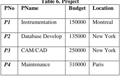
[image:4.595.320.537.130.262.2]

An experiment has been carried out to test the working of proposed Vertical Partitioning algorithm SBPA. It has been carried out on a system with core i3 processor, 3GB RAM, Matlab toolbox and MS Access database. A relation with name Project has been used for partitioning. The Project relation has been stored in MS Access database as following.

Table 6. Project

PNo PName Budget Location

P1 Instrumentation 150000 Montreal

P2 Database Develop 135000 New York

P3 CAM/CAD 250000 New York

P4 Maintenance 310000 Paris

The Project relation has tested against set of four queries Q1,

Q2, Q3and Q4 generated from any of the three sites named S1,

S2 and S3.

Q1: Find the Budget from the Project where given its

identification number.

(SELECT BUDGET, FROM PROJECT, WHERE PNO=Value)

Q2: Find the Name and Budget of all Projects.

(SELECT PNAME, BUDGET FROM PROJECT, WHERE LOCATION=Value)

Q3: Find the Name of projects located at given city.

(SELECT PNAME, FROM PROJECT, WHERE LOCATION=Value)

Q4: Find the PNo and total project Budget for each city.

(SELECT PNo, SUM (BUDGET), FROM PROJECT, WHERE LOCATION=Value)

The Attribute Usage Matrix of the above queries set is as following.

Table 7. Attribute Usage Matrix Project

Query

Attribute

PNO PNAME BUDGET LOCATION

Q1

1 0 1 0

Q2

0 1 1 1

Q3

0 1 0 1

Q4

1 0 1 1

The frequency of queries Q1, Q2, Q3and Q4 at three sites has

[image:4.595.70.265.467.589.2]

considered as following.

Table 8. Frequency Matrix Project

Query

Site

S1 S2 S3

Q1

20 25 10

Q2

5 2 0

Q3

16 18 30

Q4

3 2 1

5. EXPERIMENTAL RESULT

Using the Bond Energy Algorithm proposed by Hoffer and severance in [2], Clustered Affinity Matrix is calculated from Attribute Usage Matrix Project in Table 7. and Frequency Matrix Project in Table 8. .

Table 9. Clustered Affinity Matrix Project

Attribute

PNo Budget PName Location

PNo 61 61 6 0

Budget 61 68 13 7

PName 6 13 77 71

Location 0 7 71 71

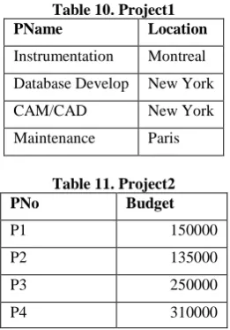
[image:4.595.323.529.492.621.2]

(5)

[image:5.595.102.233.72.259.2]

Table 10. Project1

PName Location

Instrumentation Montreal Database Develop New York

CAM/CAD New York

Maintenance Paris

Table 11. Project2

PNo Budget

P1 150000

P2 135000

P3 250000

P4 310000

6. CONCLUSION AND FUTURE SCOPE

In this paper, a Vertical Partitioning algorithm SBPA has presented and successfully implemented for improving the Query-Response-Time in Distributed Database System. The proposed algorithm SBPA has used CAM. In the first phase, CAM is calculated from AUM and FM. In the second phase, the two fragments of the relation are created by CAM Using SBPA.

The future scope of the proposed algorithm may be finding the multiple fragments of the relation.

7. REFERENCES

[1] Abuelyaman, E. S., “An Optimized Scheme for Vertical Partitioning of a Distributed Database,” in International Journal of Computer Science and Network Security (IJCSNS), Vol. 8, No. 1, January 2008, 310-316. [2] Hoffer, J.A. and Severance, D.J. 1975.The use of cluster

analysis in physical database design. In Proceedings of the 1st International Conference on Very Large Data Bases, New York, USA.

[3] Horowitz, E. and Sahni, S. 1978. Fundamentals of Computer Algorithms. Computer Science Press Rockville, Maryland.

[4] McCormick, W. T. Schweitzer P.J., and White T.W., “Problem Decomposition and Data Reorganization by A Clustering Technique,” Operation Research, Vol. 20 No. 5, September 1972, 993-1009.

[5] Navathe, S., Ceri, S., Wierhold, G. and Dou, J., “Vertical Partitioning Algorithms for Database Design,” ACM Transactions on Database Systems, Vol. 9 No. 4, December 1984, 680-710.

[6] Navathe, S. and Ra M., “Vertical Partitioning for Database Design: A Graph Algorithm,” ACM Special Interest Group on Mamagement of Data (SIGMOD)

International Conference on Management of Data, Vol. 18 No. 2, June 1989, 440-450.

[7] Chu, W. W. and Ieong, I. “A Transaction-Based Approach to Vertical Partitioning for Relational Database Systems,” IEEE Transactions on Software Engineering, Vol. 19 No. 8, August 1993, 408-412. [8] Bradley, P. S., Fayyad, U. M. and Reina, C., “Scaling

Clustering Algorithms to Large Databases”, in proceedings of the 4th International Conference on Knowledge Discovery & Data Mining , June 1998, 9-15. [9] Guha, S., Rastogi, R. and Shim, K., “CURE: an efficient

clustering algorithm for large databases”, in proceedings of the 1998 ACM SIGMOD international conference on Management of data, Vol. 27, Issue 2, June 1998, 73-84. [10] Ng, R. T. and. Han, J., “Efficient and Effective

Clustering Methods for Spatial Data Mining”, Proceedings of the 20th International Conference on Very Large Data Bases, September 1994, 144-155. [11] Jain, A. and Dubes, R., “Algorithms for Clustering

Data”, Prentice Hall, New Jersey, 1998.

[12] Kaufman, L., Rousseuw, P., “Finding Groups in Data- An Introduction to Cluster Analysis”, Wiley Series in Probability and Math. Sciences, 1990.

[13] Zhang, T., Ramakrishnan, R. and Livny, M., “An Efficient Data Clustering Method for Very Large Databases”, in proceedings of the SIGMOD international conference on Management of data, June 1996, 103-114.

8. ABOUT THE AUTHOR

Ashish Ranjan Mishra is student of Master of Technology in Department of Computer Science & Engineering at Kamla Nehru Institute of Technology (KNIT), Sultanpur, India. He has received his Bachelor of Technology degree in 2012 from College of Science and Engineering (CSE), Jhansi, India in Computer Science & Engineering.

Dr. Neelendra Badal is an Assistant Professor in the Department of Computer Science & Engineering at Kamla Nehru Institute of Technology (KNIT), Sultanpur (U.P), India. He received B.E. (1997) from Bundelkhand Institute of Technology (BIET), Jhansi in Computer Science & Engineering, M.E. (2001) in Communication, Control and Networking from Madhav Institute of Technology and Science (MITS), Gwalior and PhD (2009) in Computer Science & Engineering from Motilal Nehru National Institute of Technology (MNNIT), Allahabad. He is Chartered Engineer (CE) from Institution of Engineers (IE), India. He is a Life Member of IE, IETE, ISTE and CSI-India. He has published about 30 papers in International/National Journals, conferences and seminars. His research interests are Distributed System, Parallel Processing, GIS, Data Warehouse & Data mining, Software engineering and Networking.