Fractional Calculus for Solving generalized Abel’s
Integral Equations using Chebyshev Polynomials
M. H. Saleh
Department of Mathematics Faculty of Science, University of Zagazig
S. M. Amer
Department of Mathematics, Faculty of Science, University of ZagazigD.Sh.Mohamed
Department ofMathematics Faculty of Science, University of Zagazig
A.E.Mahdy
Department ofMathematics Faculty of Science, University of Zagazig
ABSTRACT
In this paper we investigate the numerical solution of Abel’s integral equations of the first and second kind by chebychev polynomials of the first ,second ,third and fourth kinds. Some numerical examples are presented to illustrate the method.
General Terms
Numerical solutions, Fractional integral equations
Keywords
Singular Volterra integral equation, Abel’s integral equation, Fractional calculus, Chebyshev polynomial, Collocation pionts
1.
INTRODUCTION
Abel’s integral equations provide an important tool for modeling a numerous phenomena in basic and engineering sciences such as physics, chemistry, biology, electronics and mechanics [4,14,20]. Abel’s integral equations often appears in two forms the first and second kind as follows.
And
where is a continuous function with , where T is constant. Moreover, generalized Abel’s integral equation can be considered the following forms
And
Where , , and T is constant.
The paper it organized the following way: In section , we present the fractional integral and derivative operators and some their properties. In section , we combined fractional technique, Chebyshev polynomials and the collocation method for solving Abel’s integral equation. Some examples are investigated in section . The numerical results show the
accuracy of the method. Last section is conclusion that gives some points of the method.
2.
FRACTIONAL INTEGRAL AND
DERIVATIVE
Definition 2.1.A real function , is said to be in the space , if there exists a realnumber
such that , where
and it is said to be in the space iff
,
Definition 2.2. The Riemann-Liouville fractional integral operator of order , of a function is define as
such that
proposition 2.1. The operator in definition 2.2 satisfies the following properties for ,
.
1.
2.
Definition 2.3. The Riemann-Liouville fractional derivative operator of order , of a function is define as
where means the first order derivative of .
Definition 2.4. The Caputo fractional derivative of order is define as
Where, m-1 it has the following two basic properties
and
3.
DESCRIPTION OF THE METHOD
In this method, we use the Chebyshev polynomials through the fractional calculus to approximate the solution of Abel.s integral equations. So, we introduce briefly orthogonal Chebyshev polynomials as a suitable tool for approximation [7,18].
Definition 3.1. The Chebyshev polynomial ofthe first kind for the function
is a polynomial of degree , is called Chebyshev polynomial of degree . When increase from to t decrease from to . Then the interval is domain of definition of Also, the roots of Chebyshev polynomial of degree can be obtained by the following formula
In addition, the successive Chebyshev polynomials can be obtain by the following recursive relation
Definition 3.2. The Chebyshev polynomial of the second kind for the function
is a polynomial of degree , is called Chebyshev polynomial of degree . When increase from to , t decrease from to . Then the interval is domain of definition of Also, the roots of Chebyshev polynomial of degree can be obtained by the following formula
In addition, the successive Chebyshev polynomials can be obtain by the following recursive relation
Definition 3.3. The Chebyshev polynomial of the second kind for the function
is a polynomial of degree , is called Chebyshev polynomial of degree . When increase from to , t
decrease from to . Then the interval is domain of definition of Also, the roots of Chebyshev polynomial of degree can be obtained by the following formula
In addition, the successive Chebyshev polynomials can be obtain by the following recursive relation
Definition 3.4. The Chebyshev polynomial of the second kind for the function
is a polynomial of degree , is called Chebyshev polynomial of degree . When increase from to , t decrease from to . Then the interval is domain of definition of Also, the roots of Chebyshev polynomial of degree can be obtained by the following formula
In addition, the successive Chebyshev polynomials can be obtain by the following recursive relation
Now, we apply chebyshev polynomials for solving Abel’s integral equation of the first and second kind.
3.1.
First kind
According to and , Abel’s integral equation of the first kind can be rewritten as follow
Since calculating of is directly cost and inefficient, we will use Chebyshev polynomials for approximating . We assume on interval , can be written as a infinite series of Chebyshev basis
such that will be approximated solution of Abel’s integral equation. Now, we can write in the form
Note that, we applied the linear combination property of fractional integral according to proposition . So, it is sufficient to obtain . Assume
where are coefficients of Chebyshev polynomial
of degree that are defined by Now, by replacing in we have
Proposition confirms validity of and utilizes computation of . So, substitution in gives the following form
Now, we collocate the roots of Chebyshev polynomial of degree in It leads to a system of linear equations. By solution of obtained system we have the approximate solution of Abel’s integral equation as For more efficiency of this method, we suggest reordering Chebychev series as follows
where is linear combination of . Then is reformed
This reformation leads to reduce computation the term . We remind using directly as basis instead of Chebyshev.
3.2.
Second kind
We can rewrite with consideration in the form
Similarly, we replace to So we have
or equivalently by using
After computing and substitute the collocation points we have asystem of linear equations. Solution of the system leads to the approximated solution of Abel’s integral equation. We solve some examples by this method and assess the accuracy of method in the next section.
4.
NUMERICAL EXAMPLES
This section is devoted to computational results.We apply the presented method in this paper and solve several examples. Those examples are chosen whose exact solutions exist.All of the computations have been done using the Maple 16.
Example.1. Consider Abel’s integral equation
with the exact solution . Applying chebyshev polynomials of the first kind to integral equation at , we obtain the approximate solution which is the same as the exact solution. Similarly in all caces of chebyshev polynomials.
Note : We note that if the exact solution is a polynomial of degree k, the solution is the same as the exact solution for all
Example.2.Consider the following Abel’s integral equation of the second kind
with exact solution . Similar to the previous example, Applying chebyshev polynomials of the second kind to integral equation at , we obtain the approximate solution which is the same as the exact solution. Similarly in all cases of chebyshev polynomials.
Example.3. Consider the following Abel’s integral equation of the second kind
with exact solution . The numerical results are shown in table .
with exact solution . The numerical results are shown in table .
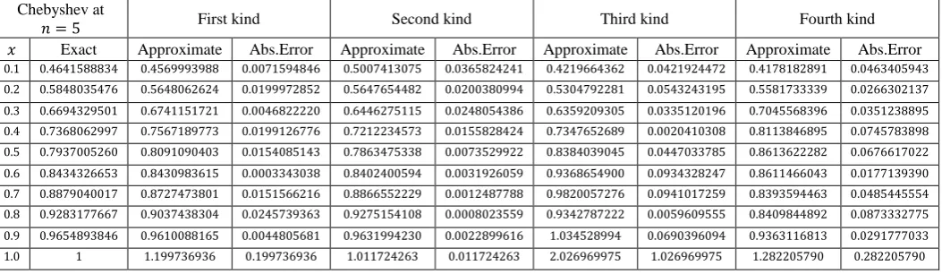
Example.5. Consider the following Abel’s integral equation of the first kind
with the exact solution . The numerical results are shown in table .
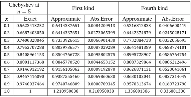
Example.6. Consider the following Abel’s integral equation of the second kind
[image:4.595.46.581.268.420.2]
with exact solution . The numerical results are shown in table .
Table 1: Estimate the exact , approximate solution and error of Example .
Chebyshev at
First kind Second kind Third kind Fourth kind
Exact Approximate Abs.Error Approximate Abs.Error Approximate Abs.Error Approximate Abs.Error
[image:4.595.50.580.440.591.2]
Table 2 : Estimate the exact , approximate solution and error of Example .
Chebyshev at
First kind Second kind Third kind Fourth kind
Exact Approximate Abs.Error Approximate Abs.Error Approximate Abs.Error Approximate Abs.Error
Table 3 : Estimate the exact , approximate solution and error of Example .
Chebyshev at
First kind Second kind Third kind Fourth kind
Exact Approximate Abs.Error Approximate Abs.Error Approximate Abs.Error Approximate Abs.Error
[image:4.595.52.579.613.766.2]
Table 4 : Estimate the exact , approximate solution and error of Example .
Chebyshev at
First kind Fourth kind
Exact Approximate Abs.Error Approximate Abs.Error
We note that the second and third kind of chebyshev polynomials are similar.
5.
CONCLUSION
In this method, we develop the Chebyshev method through the fractional calculus for solving generalized Abel's integral equations. We note that this method is easy to compute. Also, ability and efficiency of the method are great. In particular, when the exact solution of the problem is polynomial, the method gives the exact solution.
6.
REFERENCES
[1] A.A. Kilbas, H.M. Srivastava, J.J. Trujillo, Theory and Application of Fractional Differential Equations, North-Holland Mathematics studies, Vol.204, Elsevier, 2006..
[2] A.D. Polyanin, A.V. Manzhirov, Handbook of Integral Equations, CRC Press, 2008.
[3] Abbas Saadatmandia, Mehdi Dehghanb, A Collocation Method for Solving Abel's Integral Equations of First and Second Kinds,Verlag der Zeitschrift fu¨r Naturforschung,752 -- 756 (2008).
[4] C.J. Cremers, R.C. Birkebak, Application of the Abel Integral Equation to Spectrographic Data, Appl. Opt. 5 (1966) 1057-1064.
[5] G. Capobianco, D. Conte, An efficient and fast parallel method for Volterra integral equations of Abel type, J. Comput. Appl. Math. 189 (2006) 481- 493.
[6] I. Podlubny, Fractional Differential Equations, Academic Press, San Diego, CA, 1999.
[7] J.C. Mason, D.C. Handscomb, Chebyshev Polynomials, CRC Press LLC, 2003.
[8] Johin Viley, Sons ,Inc, An introduction to the fractional calculus and fractional differential equations (1993).
[9] K.B. Oldham, J. Spanier, The Fractional Calculus, Academic Press, NewYork, 1974.
[10]K.E. Atkinson, The Numerical Solutions of Integral Equations of the Second Kind, Cambridge University Press, 1997.
[11]K.S. Miller, B. Ross, An Introduction to the Fractional Calculus and Fractional Differential Equations,Wiley, NewYork, 1993.
[12]L. Huang, Y. Huang, X.F. Li, Approximate solution of Abel integral equation, Comput. Math. Appl. 56 (2008) 1748-1757.
[13]M. Rahman, Integral Equations and Their Application, WITpress, 2007.
[14]R. Estrada, R.P. Kanwal, Singular Integral Equations, Springer, 2000.
[15]R. Gorenflo, S. Vessella, Abel Integral Equations: Analysis and Applications. Lecture Notes in Mathematics 1461, Springer-Verlag, Berlin, 1991.
[16]R.K. Pandey, O.P. Singh, V.K. Singh, Efficient algorithms to solve singular integral equations of Abel type, 57 (2009) 664-676.
[17]R.P. Agarwal, D. O'Regan, Singular Differential and Integral Equations with Applications, Springer, 2003.
[18]S.A. Yousefi, Numerical solution of Abel,s integral equation by using Legendre wavelets, Appl. Math. Comput. 175 (2006) 574-580.
[19]samah M. Dardery, Mohamed M. Allan, Chebyshev Polynomials for Solving a Class of Singular Integral Equations, Applied Mathematics, 2014, 5, 753-764.
[20]T. Miyakoda, Discretized fractional calculus with a series of Chebyshev polynomial, Electron. Notes Theor. Comput. Sci. 225 (2009) 239-244.
[21]V. Mirceski, Z. Tomovski, Analytical solutions of integral equations for modelling of reversible electrode processes under voltammetric conditions, J. Electroanal. Chem. 619-620 (2008) 164-168.
[22]Z. Avazzadeh, B. Shafiee and G. B. Loghmani, Fractional Calculus for Solving Abel's Integral Equations Using Chebyshev Polynomials, Applied Mathematical Sciences, Vol. 5, 2011, no. 45, 2207 - 2216.