http://dx.doi.org/10.4236/jamp.2014.25019
How to cite this paper: Bulnes,F. (2014) Framework of Penrose Transforms on Dp-Modules to the Electromagnetic Carpet of the Space-Time from the Moduli Stacks Perspective. Journal of Applied Mathematics and Physics, 2, 150-162.
http://dx.doi.org/10.4236/jamp.2014.25019
Framework of Penrose Transforms on
D
P
-Modules to the Electromagnetic Carpet
of the Space-Time from the Moduli Stacks
Perspective
Francisco Bulnes
Department of Research in Mathematics and Engineering, TESCHA, Federal Highway Mexico-Cuautla, Tlapala La Candelaria, Chalco, State of Mexico, Mexico
Email: [email protected]
Received January 2014
Abstract
Considering the different versions of the Penrose transform on D-modules and their applications to different levels of DM-modules in coherent sheaves, we obtain a geometrical re-construction of the electrodynamical carpet of the space-time, which is a direct consequence of the equivalence
between the moduli spaces ˆ
G -equivariant
(G H C/ , ) ≅ G -equivariant(CY, ),C
M M that have been demon-
strated in a before work. In this case, the equivalence is given by the Penrose transform on the quasi-coherent Dλ-modules given by the generalized Verma modules diagram established in the Recillas conjecture to the group SO( ,1 n+1), and consigned in the Dp-modules on which have
been obtained solutions in field theory of electromagnetic type.
Keywords
Penrose Transform, Moduli Stack, Dp-Modules, Verma Modules, Field Theory, Electro-Dynamical Stacks
1. Introduction
We consider the Penrose transformation, [1] through the correspondence
F
P M
(1)
Let P, be the Penrose transform [2] associated to the double fibration (1), used to represent the holomorphic solutions of the generalized wave equation [2], with parameter of helicity
h
[3,4]:hφ = 0,
151
on some open subsets U⊂M
,
in terms of cohomological classes of bundles of lines [2], on U= ν π( −1(U)) ⊂P,
(where P,is the super-projective space).In the D-modules language the direct and inverse images of the double fibration comes given to DM-mod- ules that are DP-modules through of the right functor equivalence:
F
R ( ;Γ yOp( ))k ≅R homDY(Φ Dp(−k),OY) [ 1]y −
,
(3)where D -module transform of DP(−k), is theDM-module associated to the wave equation given in the
equa-tion (2), whose helicity is h k( )= − +(1 k/ 2).
Now in the context of the generalized D -modules (inside of the derived categories) we can use one version generalized of the Schmid-Radon transform, to cycles in the derived category and finally obtain for the Radon- Penrose Transform, the functor [5]
,
S additional geometrical hypothesis
Φ + (4)
establishing an equivalence between the category M(DX- modules / flat connection), and the category M(DY-
modules/Singularities to along of the involutive manifold V/flat connection), [2,5,6]. Then our moduli space that we constructed is the categorization of equivalences:
d[ / Y] {M( Y- modules / Singularities to along
of the involutive manifold / flat connection)
(U, )},
S D
V
H•
=
O
M
(5)
considering the moduli space as base [2,6],
d[ /S X] = {M(DX - modules / flat connection) ker(U,h k( ))},
M (6)
The additional geometrical hypothesis in the functor (4), comes established by the geometrical duality of Langlands [5], which says that the derived category of coherent sheaves on a moduli space MFlat(LG C, ), where C, is the complex given by [6]
1 -1 1 1 -1
: dj j dj j dj j di 1 j di 3
C −→E →E +→E + + →E + → , (7) which is equivalent to the derived category of D -modules on the moduli space of holomorphic vector G
-bundles given by B CG( ) [7], this shaped by the geometrical extension of a derived functor corresponding to
one Langlands ramification with corresponding stack moduli given by LBunκG [8].
Inside of this study, the transform on D -modules (see Kashiwara [9]), that arises is the Radon-Penrose transform for generalized flag manifolds in the framework of this quasi-G -equivariant D -modules (that are a class of the coherent D -modules useful in the manager of cycles to reconstruct and model the geometrical im- ages [10,11] of the electrodynamics of the space-time through of the different photon fields that interact as strings, heterotic strings and D -branes [12]), is the generalized version that we want. Likewise, in particular their Radon integral operator defines and proves the necessary invariance of the geometrical images obtained by the D -P modules transform, predicted by the Kashiwara theorem [12], and that guarantee the invariance in the solutions of the wave equation given in (2) in the frame of conformally [13] in the integral geometry context.
By the Recillas conjecture [14], and their application in the obtaining of Cěch complexes (complexes obtained in the development by derived sheaves (ver Kapustin [7])) in the tacking of strings through super-conformal spaces P
's
given in the corollary by [5], we have that the Penrose-Ward transform is done evident when the inverse images of the D -P modules that are quasi-coherent Dλ-modules established by the diagram [14](Verma modules diagram in the conjecture Recillas to the group SO(1, 1)n+ [4,15]) result naturally inside of vector bundles language as image of the degeneration of cycles given inside the manifold signed in the equiva- lences of moduli spaces in the theorem 4.1,given in [16].
Likewise the duality between string theories (string and D - branes) stay established through of the intert- wining operators of the Penrose transform and their isomorphism in all different string dualities, field/particle and the conformally and holonomy levels required in invariance of the space-time field theory.
2. Framework Penrose Transforms on
D
P-Modules that are
D
F-Modules
152
relation between them considering the corresponding intertwining operators (integral transforms that are iso-
morphism between cohomological spaces of orbital spaces [17,18] of the space-time), as for example, the twis-
tor transform to the G-orbits of the complex holomorphic bundle of the complex Riemannian manifold.
Since solutions of differential equations on manifolds and cohomological classes are part of the bases of this generalized Penrose transform, the theory of sheaf cohomology and D -modules was perfectly considered for their modern study. In [13], we used this theory to generalize and study the Penrose correspondence in (1). More recently in [15] has been studied the generalized Penrose transform between generalized flag manifolds over a complex algebraic group G, using M . The Kashiwara’s correspondence(see [14]) between quasi-G -equiva- riant-DG / H-modules and some kind representation spaces which are (g, H -) modules (loosely, they are com- plex vector spaces endowed together with an action of the Lie algebra g, associated to G, and an action of
H , which are compatible in some way) establishes the solid criteria to obtain equivalences between cohomo- logical classes when H, is a closed algebraic subgroup of G.
Conjecture. 1. [14] We want a generalization of Penrose transform on the homogeneous space
(2, ) / (1),
SL C U or a Radon transform on equivariant-D -modules on generalized flag manifolds [13,15]. Let G, be a reductive algebraic group over C, P, and Q, two parabolic subgroups containing the same Borel subgroup of G. Let X G P = / , Y G Q = / , and let S , be the unique closed G -Orbit in X×Y, for the diagonal action. Then we can identify S , with G P/ ∩Q. The natural correspondence
S Y,
X← →ν π (8)
where
ν
, and π, are the restriction to S , of the projections of X×Y, on X,and Y , induces an integral transform from X, to Y , which generalizes the classical Radon-Penrose transform. This subject has been in- vestigated intensively both in the complex and real domains (to see Baston-Eastwood [1], D’Agnolo-Schapira [6], Marastoni [11], Gindikin [13]).Our goal is to obtain one version of this transform in the framework of quasi-G -equivariant D -modules (see Kashiwara [7]), i.e. the functor
1
b b
G G *
: M ( X) M ( Y), ( ) g f ,
−
→ =
R M M R M M (9)
called the Radon transform, which is predicted by the conjecture 1, given by [15] and completed by [11], where
b G
M (M), denotes the derived category of quasi-G -equivariant D -modules with bounded cohomologies, and
*,
π and ν-1, are the operations of direct image (integration) and inverse image (pull-back) for D -modules. More precisely, we consider a D -X module of type M DL D= = X⊗OX L, where L, is an irreducible G
-equivariant locally free OX−module. In this case is had that
(R( )) 0, 0, p
H DL = ∀ <p
The Grothendieck group of the category of quasi-G -equivariant D -X modules of finite length is spanned by elements corresponding to the objects of the form DL. This means that we can generate solutions in complex holomorphic manifolds as M, through conformal solutions defined on bundle of lines, at least to each a of the derived category components of quasi-G -equivariant D -modules. From BGG-resolution and using some fact of the Dolbeault cohomology on L, discussed by Cousin complexes and their sheaves we obtain a resolution of the quasi-G -equivariant D -S module ν-1(DL), of the form:
0
-1 0
1 1
0 f ( ) 0,
n
r r
nk k
k= D k= D
→
⊕
L →→⊕
L → DL → (10)To obtain a generalization of the Kashiwara theorem in the context of the G -equivariant D -modules is necessary the geometric Zuckerman functor. This is the localization of the equivariant Zuckerman functor to the derived equivariant D -module categories on generalized flag varieties (this to apply in our study an appropri- ate D -module transform of the Penrose transform type). To this case, we define our categories of interest and construct the geometric Zuckerman functor from the basic D -module functors.
The category of (left) G -equivariant OX-module is denoted by M ( ).G X The following theorem is well
known:
Theorem 2.1. If G, acts on X, freely, there is an equivalence of categories M ( )G X ≅M(X G/ ).
153 Proof. [15].
Theorem 2.2. If X =G B/ C, there is an equivalence of categories M ( )G X ≅Re p(BC).
Proof. [15].
Let MG,a quasi-G -equivariant-DG / H-module belonging to the subcategory of DG / H−modules given by good /
M (DG H) (category of the G -equivariant-DG / H-modules).
The idea is to obtain equivalences between the different classes of DG / H−modules establishing the isomor- phism between the categories M(MG) Mod= RS( )υ
(
DG H/)
, andMG =Mgood(DG H/ ), where RS( ),υ must bethe restricted Zuckerman functor to the subcategory of left G -equivariant-DG / H-modules to obtain the de- rived category that is product of a trianguled subcategory (as the given in [16]) for a factor category that deter- mine us the Harish-Chandra functor between the categories. These equivalences in analogy to the established in (9)take the shape to the specific DG / H-modules
/ { ( / ) {derived category of / modules - - equivariants} M ( , ) M( )},
G
G H = MG DG H = DG H− G G H = MG
M g (11)
considering the moduli space as base,
/
{M( ker( , )),
equivG
G / H = DG H −modules G - equivariants U QBRST
M (12)
If we consider /
M(B\G/B) ( G H),
G= =M λ
H D ∀ λ ∈hZ*, then HG=M(B\G/B) , from the group
G=G
C
. B-equivariant D -module on the flag manifold X =G/ B,provide integral kernels and thus integral transforms, to know0
BRST
( , ) ker( , ),
H X Lλ ≅ U Q (13)
where QBRST= ∂ + Φ1 1iθ − Φ2 1iθ,such that 2
BRST 0,
Q φ= where Φ1iand
2
i
Φ , are Higgs fields on either side of the open string [7], which are implicitly these kernels?
The condition established in the kernel of equivalences inside the moduli space equivG G / H
M , is analogous to the given by the isomorphism of the Penrose transform discussed in foot of page 2, in the section 2, in [5]. The idea is extend the harmonic condition to the functions to differential operators of derived sheaves that are in BRST-cohomology, such that the equivalences in (12) are defined by certain functors due to the duality between the BGG-resolution and meromorphic version of the Cousin complex1 associated to Lλ (bundle of lines asso- ciated to the flag manifold X =G H/ , then H, is a Borel subgroup). These is the way of the classification of the differential operators with their moduli stacks. Now we will dedicate to obtain these moduli stacks to elec- tromagnetism in field theory as representation of the space-time.
3. Electromagnetic Moduli Stacks to Space-Time
A concrete application of the moduli space G/ G H
M ,on SU(2) -bundles and their complexification establishes that the moduli space of the relations between hyperbolic waves (horocycles) [18], and the Haar measure of the group action in SU(2, 2), on M,2 is the moduli space of the functors
(2) 1
0
(Hom( ( ), (2)) ( ) ( ( ( ))), , , ( ) SU j X Y
H X U
D k H D k D
D M D modules •
Γ π
= − = Φ − ∀
∈ −
P F P
P
M
where the cohomological space Hj(ΦF(DP(−k))), is the space of the SU(2)−equivariant functors related with the functors given in the relation (3) where these last come from the use of Penrose transform on D- modules [6]. But these functors are induced on orbits of SU(2, 2),conserving their equivariance through of one integral transform that relates Harish-Chandra modules from the string level like D-branes (D-modules) with one intertwining operator of cohomological description as the given in geometrical Langlands correspondence established in [8]. Then by the Langlands ramifications the moduli stack correspond to the holomorphic L
G−
bundles on C,where C, is the module defined in the complexes succession (7). Here the group L
G, is
de-1Cousin Dolbeault theory refers to the complex Dolbeault infinite dimension.
2In measurements of observables like curvature and torsion the corresponding Radon transform on spaces 4
{L L },
= ⊂
154
fined by the condition that the lattice of homomorphisms from U(1),to a maximal torus of G, be isomorphic to the weight lattice of LG.
Studies on representations to non-compactness Minkowski spaces such as that appear in electromagnetism to characterize the gauge fields in SL(2, ) /C U(1), and SU n( ), establish that when the gauge group is SU(2),
and G,is a non-compact maximal subgroup of SO(3,1), the unique non-zero invariant solutions are Abelian Maxwell fields [20]. Then this fact produces 2 0,
BRST
Q = (zero branes stability) that is to say, the D-module of
Q−branes are the torus [7] which is isomorphic to U(1).3 What is the mosaic of the field theories of the space-time in this case?
The mosaic is very simple and only includes two theories of the electromagnetic nature shaping the frame of the study Figure 1.
In this case the two different electromagnetic theories, one in the commutative case (that includes the elec- tromagnetic macroscopic fields) and other that includes the weakly electromagnetic type that conforms, joined with others considerations the gauge theory, can be the same if their semigroup operation is not invertible. To the 2−dimensional scheme of the conformation of the one only theory from two different theories (for example to the gauge −U(1)−theories) the quotients of the homogeneous space can be visualized under the Q−branes square only (blue square in the Figure 1).
We consider the description of the grading (or classification) that appears physically in terms of the U(1)R
(the re-normalizing of the group U(1)).
Considering the TQFT, and CFT, for branes and anti-branes wrapped on the entire space, the analysis from the gauge−U(1)−theories is straightforward. The tachyon T, is a degree zero operator. The term that we have that add to the boundary to describe a tachyon is the field descendant
∫
∂Σ[ , ],G T where G, is the topological- ly twisted boundary supercharge (that is to say a term in the TFT OR TQFT). The operator G, has U(1)R,charge −1, so [ , ],G T has charge −1. But a necessary condition to preserve supersymmetry is that boundary terms must be neutral under U(1)R (otherwise the U(1)R, is broken which breaks the N = 2, boundary su-
persymmetry4).
For other side, to lower dimensional sheaves, the relationship between the charge and grading is more subtle considering the dimension of the cohomological spaces to different vector bundles considered. For example, to the state corresponding to an element of Extn(S, T), for two sheaves S, and T , we need not have charge
(1)R
U , equal to n, which could be the degree of the Ext, group will not match the charge of the state. Then the use of the twistor transform results very useful until certain point when there exist correspondence between sheaves that are corresponded to mutually supersymmetric branes. For example, the inverse twistor transform applied to the sheaf O(- ),k corresponding to the
k
th
−
power of the tautological line bundle of super-projec- tive space P [21], for example the bundle of lines O(1)⊕4, when is considered a twistor-string case with 3.
P Nevertheless one important aspect that born of these relation that are explained by the twistor transform is the field consideration that gives origin to the shape of the geometry (at least in lower dimension) from the quantum states and their orbifolds visualized as the lines of their corresponding vector bundles shaping the physical stacks of the first topological electromagnetic theories to some classes of the space SL(2, ) /C U(1). But, fur- thermore using the “ramifications” to certain Langlands classes [8] we can to obtain the visualizing of the sin- gularities of the field as sources of the proper fields, through of their extensions as rational curves. Remember
Figure 1. Re-normalizing of the Group in semi-groups of electrodynamical quotients from SL(2, ) /C U(1), when QBRST2 =0 [7].
3The co-weight lattice of
,
G is defined as the lattice of homomorphisms from U(1),to a maximal torus T, of G. The weight lattice of G,is the lattice of homomorphisms from T, to U(1).
[image:5.595.230.400.568.638.2]155
that we want discomposes singular regions of the space in regions of the conformal nature that can give the val- ue of the singularity evaluated as zeros of polynomials in algebraic geometry and re-interpreted by the Penrose transform as varieties (varieties that are rational curves or algebraic curves). This is as to take a microscope and observe the flatness of the space in these singular regions (as the study frame given in the first square of the
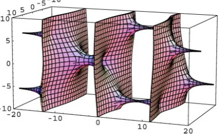
Figure 1) to these scales (for example to the QFT). To this last is very useful establish dualities between of set of equivalences from the moduli space MFlat(LG C, ), and the moduli space of the corresponding classes in (12) [5] (see Figures 2(a) and (b)).
In the case of the complexes (7) the idea is discompose a complex with non-conformal properties in “factora- ble” pieces in complexes where flatness due to the holomorphicity exists and also conformability of M, in these scales. A promissory result in that sense is the due to Kashiwara-Poicaré-Mebkhout on local cohomology where in the resolution proposed in the Bulnes corollary [14], we can investigate the cohomology5 of
P
3, through the moduli space M (P3, 0)≅P3 4. To the electrodynamical context, the moduli space is the corres- ponding to the super-projective P2 4 ≅L 4 6 (superminitwistor space).What happen in the case when the space-time group is measured from electromagnetic fields in the TQFT, or TFT contexts as SU(2)⊗T?
4. Results
As has been mentioned before, to calibrate the space-time through the electromagnetic fields is necessary re- place the Abelian group U(1), in the K−invariant G−structure of the principal
G
−
bundle ofM
, given by SG( ),M for the non-Abelian group SU(2), since we want to realize an action through electromagneticfields on a representation of the space-time given as SU(2)⊗T, where T, is the torus T≅U(1). Then
(4) (2)
SO ≅SU ⊗T, where SO(4), is a compact group of GL4.
For the isomorphism with SO(4), a representation through of U(1)−connections of the space-time will comes given for representations of the group SU(2)⊗T. An example of the application of these representa- tions is the 2−dimensional hyperbolic space whose curvature can represents through the value of certain G−
invariant integrals on lines of a bundle of lines on the principal G−bundle of U(1), and whose that come from of the relation between co-cycles of the cohomology of G L/ ,with L,an open orbit and fields of G K/ , (for example, the fields on horocycles as solutions of the wave equation on the hyperbolic plane when G=SU(1,1),
and K =SO(2)). The case that interest us is consider a G L/ , as flag manifold and with G=SL(2, ),C and .
L=T Here G K/ , is a 3−dimensional hyperbolic space.
The way to define the corresponding moduli stacks of electromagnetic nature is consider the following impli- cations that are consequences of cohomology of derived sheaves of D -F modules using the Cousin cohomology on SU(2)−bundles [8] and after extend them to the complex case:
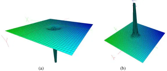
(a) (b)
Figure 2. Mirror equivalences to sources and holes of the quantum electro- magnetic fields. The first image corresponds to the hole or singularity of the
(1)
U −connections. The two images correspond to the source of the gauge
(1)
U
− −field. Both geometrical objects are equivalent inside of the dualities of the moduli spaces Flat( , ),
LG C
M and Hitchin moduli space MH( , ).G C
[image:6.595.171.459.503.625.2]156
ˆ
Cohomology of Cech Cohomology
Complexification of the Twistor model to Space - Time ˆ
hyper - functional of Cech,
→ ∂ − →
→
(14)
But this only can be realized directly through of different classes of the U(1)−bundles of the space
(2, ) / (1),
SL C U that can be given only on those states inside the Lorentz norm.
Then by ingredients from the field theory we have that the Penrose transform gives the following identifica- tion:
2( , 2 2) {hyperfunctions fields on , of helicity },
H P h− = M h (15)
But this space is too large to our purposes of field theory since it contains states of infinite norm like many radiative interactions that come from the background.
Then we consider the cohomological space
1
( , 2 2) {real analytic fields on , of helicity },
H P h− = M h (16)
which, using the positive/negative frequency decomposition due the standard polarization takes the form
1( , 2 2) 1( , 2 2).
H P+ h− ⊕H P− h−
Then by the extension of functors given in the category [8], M(sl2,SU(2)), we have
equivariant
(1), (2) (1), (2)
(R ( ( ))) R ( ),
j P
U SU U SU
H Γ DV = Γ V (17)
,
j +
∀ ∈Z and V , a Harish-Chandra module, where RPΓU(1),SU(2)( ),V is an equivariant image of the functor
modulo U(1), given in the moduli space M0, and these are the functors R ( ;Γ yOF( ))k , of the derived cate- gory D( )V .Observe the D -P modules as D -F modules inside of the sheaf OF( )k , that is to say, we want do correspond D -P modules that come from a derived sheaf to certain class branes. These branes must be that come from of the electromagnetic fields to our research.
Theorem (F. Bulnes) 4.1. [2]. The following isomorphism is valid
quasi- -equivariantG (G H C/ , ) quasi- -equivariantG ( Y, ),C C ∧• ≅
M M
being C∧•, a Cousin Dolbeault complex
-1
, , [ k/ Xk ](M)[ ] ( ( I( ))).
n p n p
X X
H R k H R
•⊗ O ≅ •⊗ O λ
E D E D
Proof. [5,24].
From the before theorem given in [5,8] we can give the application to a geometric electrodynamical represen- tation of the space-time considering conformally invariant two-dimensional theories6:
Theorem (F. Bulnes). 4.2. Using the isomorphism between the moduli space MG-equiv(CY C, )ˆ and the mod-
uli space to the stack n
λ⊗ Ω
L , we can obtain the moduli stacks 4
2
[C Z/ ].7
We want χG Hom T( , )
×
= C , [23] and obtain a result in real form spaces because we want use U(1)−gauge theory, that is to say, “Abelianize” the SU(2)−theory to find a decorated of the moduli stack where we can use the D−branes to tack the field carpet as a 2−image of the corresponding CFT-space (crystal field theory- space) obtained of the corresponding U(1)−gerbe8 [7]:
via a homomorphism Hom( ( ), (1))Z G U , to know;
( ) (1)
2 2
( , ( )) Z G U ( , (1)),
H X Z G →− H X U (18)
Proof. Considering the twistor transform that appears in the composition P T , [22] we have the Penrose
6Usually that stack is presented as
[X/C×],where to this presentation one associates a non-conformally invariant two-dimensional theory of the U(1)−gauged sigma model. As stacks they are the same: 4
2
[C Z/ ] [= X/C×]. 7For example considering a decomposition given by
2
(4) (2) (2) / .
SO =SU ⊕SU Z
8
A grebe is a construct in homological algebra and topology. A gerbe on a topological space X, is a stack G,of groupoids over X which is locally non-empty (each point in X,has an open neighbourhood U,over which the section category G U( ), of the gerbe is not empty) and transitive (for any two objects σ,and τ,of G U( ),for any open set U,there is an open covering { } ,Vi i of U, such that the
157
transform as a map congruent with Z G( ), modulo
Z
2. The congruence of these maps defines the gerbe de- fined in (18) and shapes the composition of bundles [7,21,22]9exp
0→ →Z EX →EX∗ →1, (19)
where EX∗ , is the sheaf of the smooth invertible functions on X. Of this way the co-cycles obtained by the Pe- nrose transform are Čech 1−co-cycles that come from the smooth principal U(1)−bundle. The space EX, is a fine sheaf such that 2
( , X) 0.
H X E = Thus a principal U(1)−bundle is a geometrical realization of one element of the cohomological space 1
( , X).
H X E∗ But we need establish the isomorphism between the moduli spaces
Flat( , ),
L
G C
M to D−modules and (M ( , ),G C ωK), of A−branes such and as is necessary to apply the
geometrical Langlands correspondence between of the LBunG (bundles characterized on C) and the structure sheaves like the given in O( )B (with B, a Hitchin base given by the cone 0
( , ( C) / W)
H C t×ω )10 to the bo-
sonic moduli space that we want (remember SU(2), is the electromagnetic group of weak interactions such as
0
,
W W+,H). Remember that we want obtain a photonic carpet as a U(1)R− carpet of the space-time.
Then to the Čech 1−co-cycles we need that come from holomorphic U(1)−bundles. Then the correspond- ing sheaf of inverfible holomorphic functions on X, will be X.
∗ O
Then a geometrical realization of a 0−gerbe is the cohomological group 2
( , X).
H X O∗ 11 But the 0−gerbe corresponds to a principal U(1)−bundle (in this case a gerbe equal to S1−bundle with connection) where their topological realization is a cohomological space 2
( , ).
H X Z Then considering the twisted image of this cohomological space we obtain a characteristic class of gerbe in the space 2
( , ( ))
H X Z G which is the pre-im-
age of the Penrose transform
{
}
2 2 1
( , ) ( , ) / , ( , )
H X O ≅ Φ ∈ ΓU Ω Φ =d
θ θ
∈ ΓU Ω (20)in the stack LBunG. But we want extend the electromagnetic field solution to the stacks such that ˆ
Higgs Bun ,
L L
G =T G (21) But our moduli space of the corresponding stack moduli must be the orbifolds in Ω ⊗n L , since we want
field extensions given by the Higgs field Φ ∈ Γ(L⊗Q). Different bundles implies fields that have different zero modes, which implies different anomalies which implies different physics measured from the electromagnetic gauges. All these different field physics obtained are ramifications of the same field following different patrons given by C→ ×C B. For example on a non-compact worldsheet (see the Figure 3), the instantons that have charge 1 / ,k corresponding to electrons with charge k, and massive particles can appear with periodicity es- tablished by the closed forms whose cohomological classes lands in lattice
2 2
( , 2 ) dR( ),
H Σ πRZ ≤H Σ (22) Then the Čech 1−cocyles are 1 1
( , ),
H X S who represents the kernel Z G( ), of the map (18) which is the space of the flat bundles, that is to say, the moduli space MFlat(LG C, ), who is image of the functor of finite range12
9In this point we have in the flat complex space that
a
in in 4
[1] a ab[1] ,
O → →T T →∇ O ≅ M
C C
which is conformally invariant (since the vector bundles of C, in M, need of the twistor space deduced to the derived wave operators of the affine connections let be conformally invariants). Then considering the corresponding to the forms to curved case (∇ ∇a bφ,such that (∇ ∇ − ∇ ∇a b b a) ,φ is the curvature of T (essentially the Weyl curvature of M)∀φ, a 0-form inU(1)) we find an analogous connection to 2-forms, proving the obtaining of elements of the space 2
( ).
Ω M In this composition Ta, is a twstor image of bundle using the connection
a
∇ . Then by the Penrose transform there is isomorphism between respective vector bundles. But from the congruence between (18) and
their Penrose transform P T, we have a stack modulo Z2.
10W, is the Weyl group.
11This cohomological space to all space-time M, must be 2
( , (1)),
H
M
U accord with the map (18). 121
π , is the homomorphism given by π π1= 0(Higgs). Also is explicitly given to this case (Higgs fields) by the map
0 1
( , )
( , )
H
Higgs
G C X
158
Figure 3. D−branes Moduli Stack [X/C×], calculated
with the action of C×, on Σ, lifting to an action ,
C→ × ΣC where usually to the Riemannian surface ,
Σ we can consider the causal structure of M. The phy sics are different and are corresponded to different “tim
es” ,t by a phase t τ t τ
. The different physics can
be viewed as sources (charges), holes (scattering or mas sive particles), warm holes (perturbative spaces), flat sp aces (de Sitter regions, for example ∞ −neighborhoods in Lorentzian manifolds).
2 2
1
(Hom( ( ), (1))) ( , (L )),
H Z G U H C π G
Γ ≅ (23)
But the MO-duality implies that the moduli spaces MFlat(LG C, ), and MH( , ),G C (with symplectic struc-
ture ωK ) are a mirror pair [25]. Then the flat B-fields from MH( , ),G C take values in the space
2
( , ( )) ( )
H C Z G =Z G . But is well known that Z G( ) is naturally isomorphic to π1(LG). Newly by the argu-
ments of the MO-duality we can map the class w∈Z G( ), defining the
B
-
field on MH( , ),G C to the cor-responding element in 1(L )
G
π , labeling the connected component of MH(LG C, ), (and vice versa). Then to our case when G=SU(2),then the moduli space MH( , ),G C is connected and has two possible flat
B
-fields labeled by Z SU( (2))=Z2. Then, for other side lG=SU(2) /Z2, and therefore MH(LG C, ), haves two components labeled by π1(LG)=Z2.
Finally the sheaf of the open-string states (states that come from the D−branes) is the sheaf of holomorphic functions on MH( , ),G C in the complex structure of the symplectic complex structure ωI =ωJ +iωK
13. Then
( , ),
H G C
M can be identified with MHiggs( , )G C , which the bosonic moduli space that we want.
Example 4.1. We consider the Abelian Hodge theory approach, and let LocLG( )C , with C, the curve of their corresponding ramification with the same geometry to construct the pair or Langlands data (M, ),δ where
Higgs
Bun ,
M = and
1 Higgs /
:M M B,
δ → ⊗ Ω (24)
This connection is a meromorphic relative flat connection acting along of fibers of the Hitchin map:
Higgs
: Bun ,
h →B (25)
Furthermore by construction the bundle with connection (M, ),δ is a Hecke eigen D−module with eigen- value ( , ),E ∇ (as the found in [8]) but with respect to an Abelianized version
13Since has been used the Hitchin base (to involve a the torus t, and relate the symplectic form
K
ω with ωC. Then the isomorphism given by the Penrose transform must be (because we want include the Hitchin base to singularities of the field seen these as sources or holes)
2( , n ) ker( , ),
H M Ω ⊗L ≅ U ∂ +Q where ∂ +Q, is the new connection considering the Langlands parameter to regularize the connection given by the global Langlands category of sheaves Loc (LG ),
×
[image:9.595.207.423.90.224.2]159
Higgs Higgs
(1), (2), (2).L iAbelian: D (Bunb , ) D (Bunb , ),
U U SO Φ O → ×CO (26)
of Hecke functors. These are defined again for i=1, 2, 3,,n−1, as integral transforms with respect to the tri- vial local system on the abelianized Hecke correspondences HG, λ, with BunHiggs, and BunHiggs×C, in the classic scheme of the double fibration of the integral geometry (Penrose transforms!) on micro-local objects of these bundles. Their stack moduli is LHiggs.
Corollary (F. Bulnes) 4.1. An 2−dimensional A−brane model of the electromagnetic carpet is given by
the moduli space MHiggs( , ),G C with 2d−dimension with d =1, and charge e such that,
2
1
( ).
I C
Tr A A e
ω =
∫
δ ∧δ −δφ δφ∧ (27)Proof. Applying [26], and considering the example 4.1, with the moduli space MHiggs( , ),G C with the hypo-
thesis given for our corollary, the image under the Penrose transform on double fibration in BunHiggs×C, that is to say, for example, the cohomological space H1(TP', 2h−2), (this formulation is through the integral geome-
try) can establish a 2-dimensional image given as fibration (not vector bundle (mini-twistor surface)) in
1
×
1CP CP [5]14. Then the 2-dimensional image of the electromagnetic carpet is the generated by the rotations and sources such as in the Figure 4.
Figure 4. Electromagnetic carpet of space-time ob-tained by quantum electromagnetic waves using the
coefficients ψ2, from the energy of the waves to quantum level [27]. The model is obtained simulating the waves in the corresponding SL(2, ) /C U(1),model, using a two-points function on the torus. Of this way, is obtained the framework using this orbital space pre-dicted by the gauge theory. In the carpet (blue surface) the nodes are states of energy φ,and lines (or routes) are the paths framework. The nodes are the singulari-ties or sources given in the Figure 2.
14 1
[image:10.595.223.403.303.577.2]160
For other way, the gauge field
A
,
can be naturally coupled to sources which are transformed to unitary re- presentations from U(1) ,R of G=SU(2). These are electrical sources, since they create a charge like a Cou-lumb charge of the form
2
, a a
A T
r
θ ≈ ρ (28)
where Ta, a=1, and dim ,G are generators of G, in the representation R,from U(1) .R Then if we con-
sider to the space-time M R
=
3×
R,
with ,r the distance from the origin in R3, and we assume that the world-line of the source is given for r=0, [7], then we can establish that magnetic sources are labeled by ir- reducible representations of different groups as U(1), (2),U SO(2).
We can establish using a path integral as the given by
exp{ ( )}
Z A I A
ν
=
∑∫
D − (29)the traces inside the symplectic structure given in (27), and draw the electro-physical carpet of the space-time with all constitutive sources “charges”. Here
ν
, is the principal G−bundle on M, where M, is the com- pact component of M. For example, to vector bundle given by ν =O(1)⊕4, which is basically the functor image Γ(L⊗Q), (that appeared in the demonstration of the theorem 4.2) necessary to represent the space-time
in their string 4d− model. Note that in QFT one sums over all isomorphism classes of
ν
.It’s necessary the BRST-cohomology and the equivalence between QFT, with a re-interpretation in graph quantum theory using the string theory with a photon of the class of the boson field as calculated by
( ⊗Q)
Φ ∈ ΓL . Joining the paths of this bosonfloor we obtain the corresponding Q−fields to every instanton in path integral as given by [7]
3
exp{ Qj}
j
Z A A A i
ν
=
∑
∫
D D D∑
ℑ (30)having the transformation
exp{ / 2} , a exp{ / 2} / a, exp{ } / ,
a a
Q → − Φi Q Q → − Φi Q iΦ =τ τ (31)
Then the three actions contemplated in (30) are consigned in (Qa+Qa+exp{iΦ}) [7].
From the corollary 4.1, and the before discussion with the frame (31) we have the following electromagnetic carpet and the corresponding their framework.
5. Conclusions
Develop a electromagnetic theory of space-time is equivalent to extend the electromagnetic forces to the gauge context using the concepts as supersymmetry from the conformality and holonomicity of the electromagnetic fields always present from the bosonic symmetry generators given from the dualities of the moduli spaces
Flat( , ),
L
G C
M and MH( , ).G C using their corresponding physical stacks that comes from their connections
with ramifications [8].
Using the hypothesis of that all singularities of the space-time M, are sources in different moduli stacks (mirror theory) of a Calabi-Yau manifold of the space-time M, corresponding to the superprojective flat spaces
, n m
P [5,14], we have that in their super-mini-twistor spaces the flatness is traduced in superconformality to these spaces, and their line integrals give the values of the singularities. The singularities co-shape varieties of different degrees of genus.
161
Figure 5. Hyperbolic flat model of the space-time with one singularity of space (could be one diagram in Fig- ure 4 or 6) This model is product of two orbital spaces [17,28], and conform the surface of photon back-reac- tion in presence of singularity, this visualized as a su- per-massive particle. This simulation is shaped for com- plex hyperbolic surface z x y( , )=(1 / 1.9) tanh(2 / )x y [14, 27]. The massive particle corresponds to the sources of photons and these are their nodes in the Figure 4, cor- responds to the energy states average given by the path integrals that connect them. Every node of energy that appears in the electromagnetic framework is the singu- larity of the hyperbolic space used by the twistor trans- form [21], and their neared space to the link-wave in Feynman diagrams in Figure 6, is the surface that is showed.
Figure 6. From the way established in the Figure 4, is obtained the framework using this orbital space pre- dicted by the gauge theory. In the carpet (blue surface) the nodes are states of energy φ, and lines (or ruts) are the paths framework.
manner to obtain the electromagnetic field carpet that we want. The Theorem 4.2, is the first intent through the elements and methods of the integral geometry to obtain different geometrical models, considering different electromagnetic interactions or adding they until to arrive to the curved case, which will can be included consi- dering the bundle M
→
S
4.
Acknowledgements
Thanks to the TESCHA and the State of Mexico Government for the financial support to this research work.
References
[image:12.595.211.416.424.518.2]162
York. http://dx.doi.org/10.1007/BF01942327
[2] Eastwood, M.G., Penrose, R. and Wells, R.O. (1981) Cohomology and Massless Fields. Communications in Mathe-matical Physics, 78, 305-351.
[3] Penrose, R. (1969) Solutions of the Zero-Rest-Mass Equations. Journal of Mathematical Physics, 10, 38-39.
http://dx.doi.org/10.1063/1.1664756
[4] Bailey, T.N. and Eastwood, M.G. (1991) Complex Para-Conformal Manifolds Their Differential Geometry and Twis-tor Theory. Forum Mathematicum, 3, 61-103. http://dx.doi.org/10.1515/form.1991.3.61
[5] Bulnes, F. (2013) Penrose Transform on Induced DG/H-Modules and Their Moduli Stacks in the Field Theory. Advan- ces in Pure Mathematics, 3, 246-253.
[6] D’Agnolo, A. and Shapira, P. (1996) Radon-Penrose Transform for D-Modules. Journal of Functional Analysis, 139, 349-382. http://dx.doi.org/10.1006/jfan.1996.0089
[7] Kapustin, A., Kreuser, M. and Schlesinger, K.G. (2009) Homological Mirror Symmetry: New Developments and Pers- pectives. Springer. Berlin, Heidelberg.
[8] Bulnes, F. (2013) Geometrical Langlands Ramifications and Differential Operators Classification by Coherent D-Mo- dules in Field Theory. Journal of Mathematics and System Sciences, 3, 491-507.
[9] Kashiwara, M. (1989) Representation Theory and D-Modules on Flag Varieties. Astérisque, 173-174, 55-109. [10] Helgason, S. (1999) The Radon Transform. Birkhauser Boston, Mass. http://dx.doi.org/10.1007/978-1-4757-1463-0
[11] Marastoni, C. and Tanisaki, T. (2003) Radon Transforms for Quasi-Equivariant D-Modules on Generalized Flag Manifolds. Differential Geometry and its Applications, 18, 147-176. http://dx.doi.org/10.1016/S0926-2245(02)00145-6
[12] Mason, L. and Skinner, D. (2007) Heterotic Twistor-String Theory. Oxford University.
[13] Gindikin, S. Penrose Transform at Flag Domains. The Erwin Schrödinger International Institute for Mathematical Physics. Boltzmanngasse 9, A-1090, Wien Austria.
[14] Bulnes, F. (2011) Cohomology of Moduli Spaces in Differential Operators Classification to the Field Theory(II). Pro-ceedings of FSDONA-11 (Function Spaces, Differential Operators and Non-linear Analysis), Tabarz Thur, Germany, 1, 001-022.
[15] Kashiwara, M. and Schmid, W. (1994) Quasi-Equivariant D-Modules, Equivariant Derived Category, and Representa-tions of Reductive Lie Groups, in Lie Theory and Geometry. Progr. Math., Birkhäuser, Boston, 123, 457-488.
[16] Bulnes, F. (2012) Penrose Transform on D-Modules, Moduli Spaces and Field Theory. Advances in Pure Mathematics,
2, 379-390. http://dx.doi.org/10.4236/apm.2012.26057
[17] Bulnes, F. (2013) Orbital Integrals on Reductive Lie Groups and Their Algebras. Intech, Rijeka, Croatia.
http://www.intechopen.com/books/orbital-integrals-on-reductive-lie-groups-and-their-algebras/orbital-integrals-on-red uctive-lie-groups-and-their-algebrasB
[18] Ratcliffe, J.G. (2006) Foundations of Hyperbolic Manifolds, Graduate Texts in Mathematics. 2nd Edition, 149, Sprin- ger-Verlag, Berlin, New York.
[19] Bulnes, F. (2009) Design of Measurement and Detection Devices of Curvature through of the Synergic Integral Opera- tors of the Mechanics on Light Waves. ASME, Internal. Proc. Of IMECE, Florida, 91-102.
[20] Antoine, J.P. and Jacques, M. (1984) Class. Quantum Grav., 1, 431. http://dx.doi.org/10.1088/0264-9381/1/5/002
[21] Dunne, E.G. and Eastwood, M. (1990) The Twistor Transform. In: Bailey, T.N. and Baston, R.J., Eds., Twistor in Mathematics and Physics, Cambridge University Press, 110-127.
[22] Bulnes, F. (2006) Doctoral Course of Mathematical Electrodynamics. Internal. Proc. Appliedmath, 2, 398-447.
[23] Ben-zvi, D. and Nadler, D. (2011) The Character Theory of Complex Group.
[24] Mebkhout, Z. (1977) Local Cohomology of Analytic Spaces. Rubl. RIMS, Kioto, Univ., 12, 247-256.
[25] Hausel, T. and Thaddeus, M. (2003) Mirror Symmetry, Langlands Duality and the Hitchin System. Inventiones Mathe- maticae., 153, 197-229. http://dx.doi.org/10.1007/s00222-003-0286-7
[26] Bershadsky, M., Johansen, A., Sadov, V. and Vafa, C. (1995) Topological Reduction of 4-d SYM to 2-d Sigma Models. Nuclear Physics B, 448, 166. http://dx.doi.org/10.1016/0550-3213(95)00242-K
[27] Weylman, H. (2012) Path Integrals for Photons: The Framework for the Electrodynamics Carpet of the Space-Time. Journal on Photonics and Spintronics, 1, 21-27.
[28] Bulnes, F. (2012) Electromagnetic Gauges and Maxwell Lagrangians Applied to the Determination of Curvature in the Space-Time and their Applications. Journal of Electromagnetic Analysis and Applications, 4, 252-266.

![Figure 4. Electromagnetic carpet of space-time ob-tained by quantum electromagnetic waves using the coefficients quantum level [27]](https://thumb-us.123doks.com/thumbv2/123dok_us/8036435.770291/10.595.223.403.303.577/figure-electromagnetic-carpet-tained-quantum-electromagnetic-coefficients-quantum.webp)

