Complex Dynamics of Jungck Ishikawa Iterates for Hyperbolic Cosine Function

(1)

Complex Dynamics of Jungck Ishikawa Iterates for

Hyperbolic Cosine Function

Suman Pant

Research Scholar G. B. Pant Eng. College,

Pauri Garhwal

Yashwant S. Chauhan,

Ph.D

Assistant Professor G. B. Pant Eng. College,

Pauri Garhwal

Priti Dimri,

Ph.D

Asso. Professor and Head G. B. Pant Eng. College,

Pauri Garhwal

ABSTRACT

The dynamics of transcendental function is one of emerging and interesting field of research nowadays. We introduce in this paper the complex dynamics of hyperbolic cosine function of the type {cosh (zn ) + z + c = 0} and applied Jungck Ishikawa iteration to generate new Relative Superior Mandelbrot set and Relative Superior Julia set. In order to solve this function by Jungck –type iterative schemes, we write it in the form of Sz = Tz, where the function T, S are defined as Tz = cosh( zn ) +c and Sz = - z. Only mathematical explanations are derived by applying Jungck Ishikawa Iteration for transcendental function in the literature but in this paper we have generated relative Mandelbrot sets and Relative Julia sets.

Keywords

Complex dynamics, Relative Superior Mandelbrot set, Relative Julia set, Jungck Ishikawa Iteration

1. INTRODUCTION

The study of dynamical behavior of the transcendental functions was initiated by Fatou [12]. For transcendental function, points with unbounded orbits are not in Fatou sets but they must lie in Julia sets.

In complex analysis, the hyperbolic functions arise as the imaginary parts of sine and cosine .When considered defined by a complex variable, the hyperbolic functions are rational functions of exponentials, and are hence meromorphic.

In this past literature the cosine function was considered of the following forms:

(i) cos (zn) + c = 0 (ii) (cos z + c)n = 0 (iii) acos(zn)+c=0 (iv) (acos (z) + c)n = 0

But now we have used hyperbolic cosine function of the type cosh(zn) + z + c = 0 where n



2 and applied Jungck Ishikawa iterates to develop fractal images of this transcendental function. Escape criteria of polynomials are used to generate Relative Superior Mandelbrot Sets and Relative Superior Julia Sets. Our results are different from existing results in literature.

2. PRELIMINARIES

The process of generating fractal images from z cosh (zn

) + z + c is similar to the one employed for the

self-squared function [17]. Briefly, this process consists of iterating this function up to N times.

Starting from a value z0 we obtain z1, z2, z3, z4 ... by applying

the transformation z cosh(zn

) + z + c

2.1 Ishikawa Iteration [8]

Let X is a subset of real or complex numbers and T: X→ X for x0∈ X, we have the sequences {xn} and {yn} in X in the

following manner:

x n+1 = αn T y n + (1- α n ) x n

y n = βn T x n + (1- β n ) x n

where 0 ≤ βn ≥ 1 and 0 ≤ αn ≥ 1 and αn & βn both convergent

to non zero number.

2.2 Definition [14]

The sequences {xn} and {yn} constructed above is called

Ishikawa sequences of iteration or relative superior sequences of iterates. We denote it by (x0, α n , β n ,t) .Notice that RSO

(x0, α n , β n ,t) with β n = 1 is RSO(x0, α n ,t) i.e. Mann’s orbit

and if we place α n = β n =1 then RSO (x0, α n , β n ,t) reduces

to O (x0, t ) .We remark that Ishikawa orbit RSO(x0, α n , β n ,t)

with β n = 1/2 is Relative superior orbit. Now we define

Julia set for function with respect to Ishikawa iterates. We call them as Relative Superior Julia sets.

2.3 Definition [14]

The set of points SK whose orbits are bounded under Relative superior iteration of function Q (z) is called Relative Superior Julia sets. Relative Superior Julia set of Q is a boundary of Julia set RSK.

2.4 Jungck Ishikawa Iteration [16]

Let(X, ║.║) be a Banach space and Y an arbitrary set. Let S, T: Y→X be two non self-mappings such that T(Y) S(Y), S(Y) is a complete subspace of X and S is injective. Then for xo ∈Y, define the sequence {S x n }iteratively by

S x n+1 = α n T y n + (1- α n ) S x n

S y n = β n T x n + (1- β n ) S x n

where 0 ≤ βn ≥ 1 and 0 ≤ αn ≥ 1 and αn & βn both convergent

to non zero number.

3. GENERATING THE FRACTALS

Fractals have been generated from , using escape-time techniques-

(2)

Suppose that |z | >max {|c |, 2 /s , 2 /s ' }, then |zn| >(1+λ) n|z | and |zn|→∞ as n →∞ . So, |z | ≥ c |, and

|z |>2/s as well as |z |>2/ s ' shows the escape criteria for quadratics.

3.2 Escape Criterion for Cubics[14]

Suppose that |z | >max {|b | , (a+ 2 /s) ½ , (a+ 2 /s ') ½ }, then |zn|→∞ as n →∞ .This gives the escape criteria for cubic

polynomials.

3.3 General Escape Criterion [14]

Suppose that |z | >max {|b | , (a+ 2 /s) ½ , (a+ 2 /s ') ½ }, then |zn|→∞ as n →∞ is the general escape criteria.

4. FIXED POINTS

[image:2.595.309.549.72.171.2]

4.1 Fixed points of quadratic function

Table 1: Orbit of F (z) for (zo= -0.8125-0.1125i) at



=0.5,



=0.5, c=0.1

No. of iterations

|Tz| No. of iterations

|Tz|

1 1.30289 11 1.32199

2 1.31711 12 1.32223

3 1.32285 13 1.32217

4 1.32199 14 1.32219

5 1.32223 15 1.32219

6 1.32217 16 1.32219

7 1.32199 17 1.32219

8 1.32223 18 1.32199

9 1.32217 19 1.32223

10 1.32219 20 1.32217

Here we observe that the value converges to a fixed point 1.32219 after 6 iterations.

Figure 1: Orbit of F (z) for (zo= -0.8125-0.1125i) at



=0.5,



=0.5, c=0.1

Table 2: Orbit of F (z) for (zo= -2.6875-0.0625i) at



=0.8,



=0.1, c=0.1

No of

Iterations |Tx|

No of

Iterations |Tx|

71 74.025 86 1.1217

72 1.1217 87 74.0253

73 74.0256 88 1.1217

74 1.1217 89 74.0253

75 74.0251 90 1.1217

76 1.1217 91 74.0253

77 74.0255 92 1.1217

78 1.1217 93 74.0253

79 74.0252 94 1.1217

80 1.1217 95 74.0253

81 74.0254 96 1.1217

82 1.1217 97 74.0253

83 74.0253 98 1.1217

84 1.1217 99 74.0253

85 74.0254 100 1.1217

[image:2.595.335.527.231.383.2]

Here we 70 iterations and observed that the value converges to two fixed points 74.0253 and 1.1217 after 87 iterations.

Figure 2. Orbit of F (z) for (zo= -2.6875-0.0625i) at



=0.8,



=0.1, c=0.1

Table 3: Orbit of F (z) for (zo=-0.35625-1.65i) at



=0.3,



=0.7, c=0.1 No. of

iterations |Tz|

No. of

iterations |Tz|

1 6.71552 11 1.26349

2 1.99943 12 1.26342

3 1.21717 13 1.26339

4 0.88466 14 1.26338

5 1.13628 15 1.26338

6 1.26549 16 1.26338

7 1.26856 17 1.26338

8 1.26571 18 1.26338

9 1.26426 19 1.26338

10 1.26370 20 1.26338

Here we observed that the value converges to a fixed point 1.26338 after 13 iterations.

0 10 20 30 40 50 60 70 80 90 100

-0.813 -0.812 -0.811 -0.81 -0.809 -0.808 -0.807 -0.806 -0.805 -0.804

0 10 20 30 40 50 60 70 80 90 100

[image:2.595.67.265.441.590.2]

(3)

Figure 3: Orbit of F (z) for (zo=-0.35625-1.65i) at



=0.3,



=0.7, c=0.1

[image:3.595.72.263.80.231.2]

4.2 Fixed points of cubic function

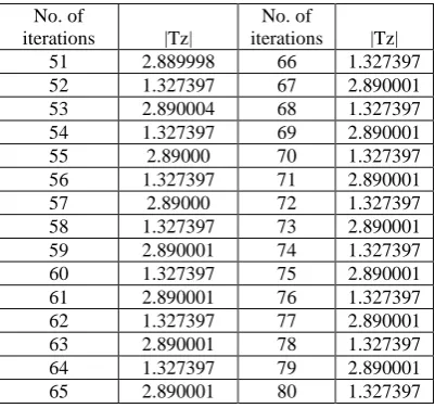
Table 1: Orbit of F (z) for (zo=-0.9+1.04375) at



=0.5,



=0.7, c=0.1

No. of

iterations |Tz|

No. of

iterations |Tz|

51 2.889998 66 1.327397

52 1.327397 67 2.890001

53 2.890004 68 1.327397

54 1.327397 69 2.890001

55 2.89000 70 1.327397

56 1.327397 71 2.890001

57 2.89000 72 1.327397

58 1.327397 73 2.890001

59 2.890001 74 1.327397

60 1.327397 75 2.890001

61 2.890001 76 1.327397

62 1.327397 77 2.890001

63 2.890001 78 1.327397

64 1.327397 79 2.890001

65 2.890001 80 1.327397

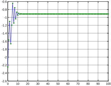
[image:3.595.331.517.115.305.2]

Here we skipped 50 iterations and observed that the value converges to two fixed points 2.890001 and 1.327397 after 58 iterations.

Figure 1: Orbit of F (z) for (zo=-0.9+1.04375) at



=0.5,

[image:3.595.331.524.356.506.2]



=0.7, c=0.1

Table 2: Orbit of F (z) for (zo=-1.31875+1.1225i) at



=0.3,



=0.5, c=0.1

No. of iterations

|Tz|

11 1.3534 26 1.3392

12 1.3127 27 1.3384

13 1.3605 28 1.3388

14 1.3293 29 1.3387

15 1.3381 30 1.3386

16 1.3445 31 1.3388

17 1.3322 32 1.3386

18 1.3431 33 1.3387

19 1.3373 34 1.3387

20 1.3379 35 1.3387

21 1.3404 36 1.3387

22 1.3372 37 1.3387

23 1.3395 38 1.3387

24 1.3386 39 1.3387

25 1.3384 40 1.3387

Here we skipped 10 iterations and observed that the value converges to a fixed point 1.3387 after 32 iterations.

Figure 2: Orbit of F (z) for (zo=-1.31875+1.1225i) at



=0.3,



=0.5, c=0.1

Table 3: Orbit of F (z) for (zo = -1.925-1.7375i) at



=0.3,



=0.2, c=0.1

No of Iterations

|Tx| No of Iterations

|Tx|

1 14879.0392 16 1.60569

2 17.11398 17 1.60569

3 1.50879 18 1.60566

4 4.78429 19 1.60567

5 1.53148 20 1.60567

6 1.47782 21 1.60567

7 1.66984 22 1.60567

8 1.60781 23 1.60567

9 1.59224 24 1.60567

10 1.61045 25 1.60567

11 1.60660 26 1.60567

12 1.60431 27 1.60567

13 1.60601 28 1.60567

0 10 20 30 40 50 60 70 80 90 100

-0.8 -0.7 -0.6 -0.5 -0.4 -0.3 -0.2 -0.1

0 10 20 30 40 50 60 70 80 90 100

-1 -0.5 0 0.5 1 1.5 2

0 10 20 30 40 50 60 70 80 90 100

[image:3.595.71.272.357.545.2] [image:3.595.70.263.603.733.2]

(4)

14 1.60582 29 1.60567

15 1.60554 30 1.60567

Figure 3: Orbit of F (z) for (zo = -1.925-1.7375i) at



=0.3,



=0.2, c=0.1

[image:4.595.332.523.82.231.2]

4.3 Fixed points of biquadratic function

Table 1: Orbit of F (z) for (zo= -2.66875+0.00625i) at



=0.5,



=0.5, c=0.1 No. of

iterations

|Tz|

21 1.1097 36 2.1494

22 2.1476 37 1.1097

23 1.1097 38 2.1494

24 2.1485 39 1.1097

25 1.1097 40 2.1494

26 2.1490 41 1.1097

27 1.1097 42 2.1494

28 2.1492 43 1.1097

29 1.1097 44 2.1494

30 2.1493 45 1.1097

31 1.1097 46 2.1494

32 2.1493 47 1.1097

33 1.1097 48 2.1494

34 2.1494 49 1.1097

35 1.1097 50 2.1494

Here we skipped 20 iterations and observed that the value converges to two fixed points 1.1097 and 2.1494 after 32 iterations.

Figure 1: Orbit of F (z) for (zo= -2.66875+0.00625i) at

[image:4.595.69.261.145.293.2]



=0.5,



=0.5, c=0.1

Table 2: Orbit of F (z) for (zo= -1.6875+0.84375) at



=1,



=1, c=0.1

No. of

iterations |Tz|

No. of

iterations |Tz|

1 17.4696 11 1.11051

2 1.10000 12 1.11051

3 1.11399 13 1.11051

4 1.10956 14 1.11051

5 1.11078 15 1.11051

6 1.11043 16 1.11051

7 1.11053 17 1.11051

8 1.11050 18 1.11051

9 1.11051 19 1.11051

10 1.11051 20 1.11051

[image:4.595.68.256.376.578.2]

Figure 2: Orbit of F (z) for (zo= -1.6875+0.84375) at



=1,



=1, c=0.1

0 10 20 30 40 50 60 70 80 90 100

-2 -1.8 -1.6 -1.4 -1.2 -1 -0.8 -0.6 -0.4

0 10 20 30 40 50 60 70 80 90 100

-3 -2.5 -2 -1.5 -1 -0.5

0 10 20 30 40 50 60 70 80 90 100

[image:4.595.329.522.506.656.2]

(5)

[image:5.595.70.263.354.503.2]

Table 3: Orbit of F (z) for (zo = -2.24375+1.3375i) at



=0.3,



=0.2, c=0.1

No. of

iterations |Tz|

No. of

iterations |Tz|

1 58829601051.3444 16 1.3454

2 227.4253 17 1.3503

3 2.0861 18 1.3476

4 10.1152 19 1.3491

5 1.2891 20 1.3483

6 1.0992 21 1.3487

7 1.6548 22 1.3485

8 1.1541 23 1.3486

9 1.8486 24 1.3485

10 1.2591 25 1.3486

11 1.425 26 1.3485

12 1.3165 27 1.3485

13 1.3687 28 1.3485

14 1.3383 29 1.3485

15 1.3544 30 1.3485

[image:5.595.316.549.417.677.2]

Figure 3: Orbit of F (z) for (zo = -2.24375+1.3375i) at



=0.3,



=0.2, c=0.1

5. GEOMETRY OF RELATIVE

SUPERIOR MANDELBROT SETS AND

RELATIVE SUPERIOR JULIA SETS

Relative Superior Mandelbrot Sets

In case of quadratic function, the central body is divided into three parts or we can say it looks like a flower having 3 leaves. It is seen that the body is symmetric along the real axis only. Each part has one secondary lobe which is approximately equal in size.

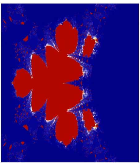
In case of cubic function, the central body is divided into 5 equal parts or we can say it looks like a flower having 5 leaves .Each part have one secondary lobe of different sizes. It is seen that the body is symmetric along the real axis only. For



=0.3,



=0.5, the size of the secondary lobes is larger as compared to other values.

In case of biquadratic function, the central body is divided into seven equal parts or we can say it looks like a flower having 7 equal size leaves. Each part having one secondary

lobe of different sizes. It is seen that the body is symmetric along the real axis only.

Relative Superior Julia Sets

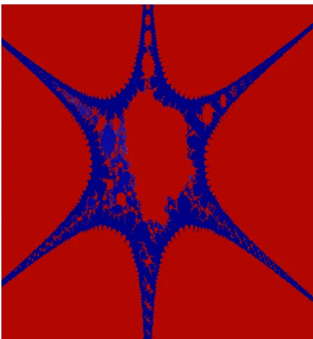
Relative Superior Julia Sets for the transcendental function cosh(z) appears to follow law of having 2n wings. These sets are symmetric along both the axes i.e. along real and imaginary axis.

For quadratic function the Relative Superior Julia Set is divided into four wings having red central body. These sets are symmetric along both the axes.

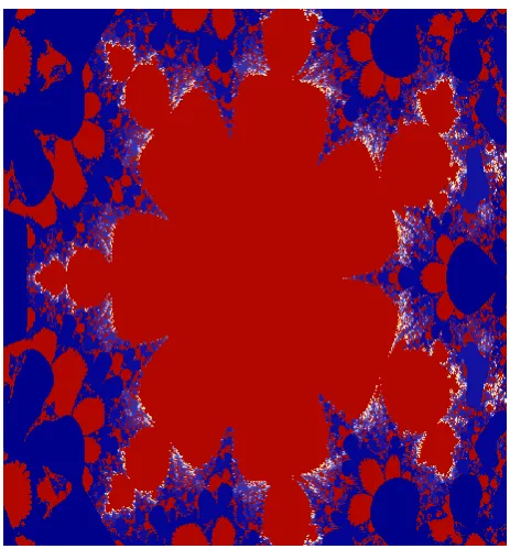
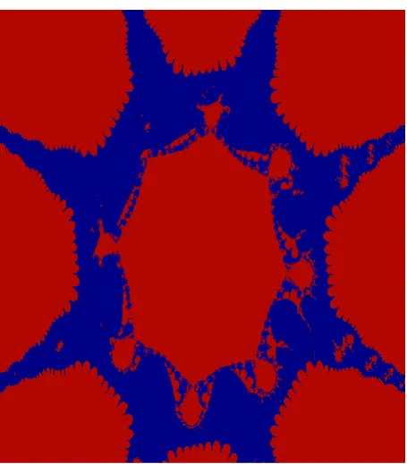
For cubic function the Relative Superior Julia Set is divided into six wings having reflectional and rotational symmetry, along with a larger red central region.

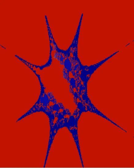
For biquadratic function the Relative Superior Julia Set is divided into eight wings possessing the reflectional and rotational symmetry and it is having a larger escape region as compared to quadratic and cubic function.

It is also observed from the graphical study of fixed points of Relative Superior Julia Sets that the convergence for



=0.5,



=0.5 and



=1,



=1 is quite fast for all polynomials in comparison to the convergence for other values.

6. GENERATION

OF

RELATIVE

SUPERIOR MANDELBROT SETS

We generated the Relative Superior Mandelbrot sets. We present here some beautiful filled Relative Superior Mandelbrot sets for quadratic, cubic and biquadratic function.

6.1 Relative Superior Mandelbrot sets for

Quadratic function

Figure 1: Relative Superior Mandelbrot Set for



=



=0.5 & c = -0.8125-0.1125i

0 10 20 30 40 50 60 70 80 90 100

(6)

[image:6.595.54.282.69.315.2] [image:6.595.317.542.107.341.2]



=0.8,

[image:6.595.54.281.358.622.2]



=0.1, c=-2.6875-0.0625i



=0.3,



=0.7, c=-0.35625-1.65i

6.2 Relative Superior Mandelbrot Sets for

Cubic function



=0.5 ,



=0.7, c=-0.9+1.04375i



=0.3,

[image:6.595.316.543.381.643.2]

(7)

[image:7.595.55.285.68.318.2] [image:7.595.318.543.73.314.2]



=0.3,



=0.2, c = -1.925-1.7375i

6.3 Relative Superior Mandelbrot sets for

biquadratic function



=0.5,

[image:7.595.325.534.352.606.2]



=0.5, c = -2.66875+0.00625i



=1,



[image:7.595.54.286.389.639.2]

=1, c = -1.6875+0.84375i



=0.3,



=0.2, c = -2.24375+1.3375i

7. GENERATION OF RELATIVE

SUPERIOR JULIA SETS

(8)

7.1 Relative Superior Julia sets for

[image:8.595.318.548.73.317.2] [image:8.595.54.285.74.330.2]

Quadratic function

Figure 1: Relative Superior Julia Set for



=



=0.5 & c = -0.8125-0.1125i



=0.8,

[image:8.595.316.540.390.632.2]



=0.1, c=-2.6875-0.0625i



=0.3,



=0.7, c=-0.35625-1.65i

[image:8.595.54.283.395.644.2]

7.2 Relative Superior Julia Sets for Cubic

function

(9)

[image:9.595.54.280.71.323.2] [image:9.595.317.544.73.323.2]



=0.3,



=0.5, c = -1.31875+1.225i



=0.3,



=0.2, c = -1.925-1.7375i

7.3 Relative Superior Julia sets for

biquadratic function

[image:9.595.317.545.364.624.2]



=0.5,



=0.5, c = -2.66875+0.00625i



=1,



=1, c =

(10)

[image:10.595.56.275.72.346.2]



=0.3,



=0.2,

c = -2.24375+1.3375i

8. CONCLUSION

In this paper we studied the hyperbolic cosine function which is one of the members of transcendental family. The fixed point 0 for S (z) = cosh (zn ) +z + c = 0 also satisfies S’ (0) = 1. Relative Superior Mandelbrot sets for the hyperbolic transcendental function cosh(z) appear like beautiful flowers having the symmetry of 2n-1 petals/leaves while Relative Superior Julia Sets appears to follow law of having 2n wings. The surrounding region of the Mandelbrot set appears to be an invariant Cantor set in the form of curve or “hair” that extends to



. The orbit of any point on hair tends to infinity under iteration. Here the geometry of hairs is quite similar to that of exponential family and hence showed the property of transcendental function. The region filled up with large number of escaping points represents Julia set plane.

9. REFERENCES

[1] Suman Joshi, Dr.Yashwant Singh Chauhan and Dr. Ashish Negi, “New Julia and Mandelbrot Sets for Jungck Ishikawa Iterates” International Journal of Computer Trends and Technology (IJCTT), vol.9, no.5, pp.209-216, 2014.

[2] Suman Joshi, Dr.Yashwant Singh Chauhan and Dr.Priti Dimri ,“Complex Dynamics of Multibrot Sets for Jungck Ishikawa Iteration” International Journal of Research in Computer Applications and Robotics (IJRCAR), vol. 2, no. 4, pp. 12-22, 2014.

[3] Suman Pant, Dr.Yashwant Singh Chauhan and Dr.Priti Dimri ,“Complex Dynamics of Sine Function using Jungck Ishikawa Iteration” International Journal of Computer Applications (IJCA), vol. 94, no. 10, pp. 44-54, 2014.

[4] E. F. Glynn, “The Evolution of the Gingerbread Mann”,Computers and Graphics 15,4 (1991), 579 -582. [5] U. G. Gujar and V. C. Bhavsar, “Fractals from z=zα

+c in the Complex c-Plane”, Computers and Graphics 15,

(1991), 441-449.

[6] U. G. Gujar, V. C. Bhavsar and N. Vangala, “Fractalsfrom z=zα+c in the Complex z-Plane”, Computersand Graphics 16, 1 (1992), 45-49.

[7] R. Chugh and V. Kumar, “Strong Convergence and Stability results for Jungck-SP iterative scheme, International Journal of Computer Applications, vol. 36,no. 12, 2011.

[8] S. Ishikawa, “Fixed points by a new iteration method”, Proc. Amer. Math. Soc.44 (1974), 147-150.

[9] G. Julia, “Sur 1’ iteration des functions rationnelles”, JMath Pure Appli. 8 (1918), 737-747

[10] B. B. Mandelbrot, The Fractal Geometry of Nature, W. H.Freeman, New York, 1983.

[11] Eike Lau and Dierk Schleicher, “Symmetries of fractals revisited.” Math. Intelligencer (18) (1) (1996), 45-51.MR1381579 Zbl 0847.30018.

[12] J. Milnor, “Dynamics in one complex variable; Introductory lectures”, Vieweg (1999).

[13]Shizuo Nakane, and Dierk Schleicher, “Non-local connectivity of the tricorn and multicorns”, Dynamical systems and chaos (1) (Hachioji, 1994), 200-203, World Sci. Publ., River Edge, NJ, 1995. MR1479931.

[14] Rajeshri Rana, Yashwant S Chauhan and Ashish Negi.Article: Non Linear Dynamics of Ishikawa Iteration. International Journal of Computer Applications 7(13):43–49, October 2010. Published By Foundation of Computer Science.ISBN: 978-93-80746-97-5.

[15] Ashish Negi, “Generation of Fractals and Applications”, Thesis, Gurukul Kangri Vishwvidyalaya, (2005).

[16] M.O.Olatinwo, “Some stability and strong convergence results for the Jungck-Ishikawa iteration process,”Creative Mathematics and Informatics, vol. 17, pp. 33-42, 2008.

[17] Peitgen, H.O., Jurgens, H. and Saupe, D., Chaos and Fractals: New Frontiers of Science. Springer-Verlag, New York, Inc, 2004.

[18] A. G. D. Philip: “Wrapped midgets in the Mandelbrot set”, Computer and Graphics 18 (1994), no. 2, 239-248. [19] Shizuo Nakane, and Dierk Schleicher, “On multicorns

and unicorns: I. Antiholomorphic dynamics. Hyperbolic components and real cubic polynomials”, Internat. J. Bifur. Chaos Appl. Sci. Engrg, (13) (10) (2003), 2825-2844.