Short Term Electrical Load Forecasting for Iraqi Power System based on Multiple Linear Regression Method

Volume 100– No.1, August 2014

Short-Term Electrical Load Forecasting for Iraqi Power

System based on Multiple Linear Regression Method

Firas M. Tuaimah

University of Baghdad Baghdad, Iraq

Huda M. Abdul Abass

University of Baghdad Baghdad, Iraq

ABSTRACT

In this paper an investigation for the short term (up to 24 hours) load forecasting of the demand for the Iraqi Power System would be presented, using a Multiple Linear Regression (MLR) method. After a brief analytical discussion of the technique, the usage of mathematical models and the steps to compose the MLR model will be explained. As a case study, historical data consisting of hourly load demand, humidity, wind speed and temperatures of Iraqi electrical system will be used, to forecast the short term load. Two models will be presented; one for winter and the second for summer season. Algorithms implementing this forecasting technique have been programmed using MATLAB and applied to the case study. This study uses the linear static parameter estimation technique as they apply to the twenty four hour off-line forecasting problem.

Keywords

Short Term Load forecasting (STLF), Multiple Linear Regression (MLR), Weather parameters.

1.

INTRODUCTION

The quality of the short-term hourly load forecasting with lead times ranging from one hour to several days ahead has a significant impact on the efficiency of operation of any electrical utility. Many operational decisions such as economic scheduling of the generating capacity, scheduling of fuel purchase and system security assessment are based on such forecasts. Short-term weather variability and, in the longer term, climate variability has a major impact on the generation, transmission and demand for electricity. Prederegulation, utilities generally managed to limit weather and climate impacts through central planning and vertical integration. In the long term, sufficient plant was planned and constructed to meet anticipated peak demand, whilst the costs arising from short-term variability were absorbed and passed on to consumers. With deregulation market participants are becoming exposed to these effects. Hence, there is greater need to manage the impact of weather and climate uncertainty. Weather is defined as the atmospheric conditions existing over a short period in a particular location. It is often difficult to predict and can vary significantly even over a short period. Climate also varies in time: seasonally, annually and on a decadal basis [1].

Weather components such as temperature, wind speed, cloud cover play a major rule in short-term load forecasting by changing daily load curves. The characteristics of these components are reflected in the load requirements although some are affected more than others. Therefore temperature, humidity and wind speed are used as variables for winter and summer seasons with historical load date to improve predict hourly load. Load demand depends on parameters such as changes in ambient temperature, wind speed, precipitation and humidity. As electricity demand is closely influenced by these climatic parameters, there is likely to be an impact on demand

patterns. Every hour load demand depends on these crucial role parameters.

As developing countries improve their standard of living, their use of air conditioning and other weather-dependent consumption may increase the demand sensitivity to climate change.

This paper attempts at first hand statistical regression methods for existing studies on parameter impacts on electricity demand and outlines how this is being assessed for the rapidly growing Iraqi electricity sector.

2.

MULTIPLE LINEAR REGRESSION

Multiple linear regressions are the earliest technique of load-forecasting methods. Here, load is expressed as a function of explanatory weather and non-weather variables that influence the load. The influential variables are identified on the basis of correlation analysis with load, and their significance is determined through statistical tests such as True and False tests. Mathematically, the load model using this approach can be written as [2]-[6]:

(1)

Where Y (t) is the load value at time t, are explanatory variables, is the residual load at time t, and (a) are the regression parameters relating the load to the explanatory variables

If the number of observations equals exactly the number of parameters to be estimated, then is forced to zero. Equation (1) becomes:

(2) The asterisk indicates the optimal estimated values of the parameters. The multiple linear regression technique has found greatest application as an offline forecasting method and is generally unsuitable for online forecasting because it requires many external variables that are difficult to introduce into an online algorithm. These models are relatively simple to apply but require extensive initial analysis to identify the repressors and their place in each model. Also, because the relationship between the load and weather variable is time specific, this model requires continuous re-estimation of its parameters to perform accurately [2].

For this forecasting study, data during the winter season and summer season were used separately. In the MLR application, the hourly load is modeled as: (i) Intercept component which is assumed constant for different time intervals of the day, (ii) Time of observation which is represent the load characteristic of the day. (iii) Temperature sensitive component which is function of difference of temperature [2], [3], [7].

in form of polynomial term. This model expresses the load at any discrete time instant (t) as a function of a base load and a weather-dependent component.

Based on early analyses, initial winter and summer models were formulated and tested in offline simulation mode [2], [3].

2.1 Winter model

Mathematically, the load at any discrete instant t, where t varies from 1 to 24, can be expressed as [2]:

(3)

Where:

= load at time = 1, 2... 24

= temperature deviation at time t.

The temperature deviation at the instant t is calculated as the difference between the dry bulb temperature at time t and the average dry bulb temperature of the previous four weekday’s temperature measurements, corresponding to the same discrete instant; that is [2]:

(4)

Where Td (t) is the dry blub temperature at time t, in °C;

Ta (t) is the average dry blub temperature at time t.

(5)

= wind-cooling factor at time t.

= base load at timet.

are the regression parameters to be estimated at time t.

The wind-cooling factor is calculated from:

W (t) = [18 – Td (t)]. [V (t)] ½ (6) Where V (t) is the wind speed in km/h at time t

2.2 Summer Model

The winter equivalent of the load model given by equation (3) can be modified for these summer model to become [2], [3]:

(7)

Where = load at time t.

= temperature deviation at time t.

= base load at time t.

are the regression parameters to be estimated at time t.

The temperature deviation is calculated as for the winter model.

The humidity factor , which replaces the wind-cooling

factor in the winter model, is given by [2], [3]:

(8)

Where is the dew-point temperature at time t, in °C Equations (3) and (7) give the multiple linear regression models for the load in winter and summer weeks. As such, this model is required to estimate (10) parameters to predict the next day's daily load profile. Equations (3) and (7) can be rewritten in compact form as:

Y (t) = f (t) X (t) (9)

Where f (t) is a fitting function given by: In winter:

(10)

And in summer:

(11)

Moreover, X (t) is the parameter’s vector to be estimated and is given by:

(12)

In this work, the parameter vector of equation (12) is assumed to be crisp (a vector with constant values at time t).

The corresponding parameters X (t) at any given discrete interval are estimated using the previous three weeks' worth of weekday data corresponding to the discrete instant. The over determined system of equations corresponding to the estimates at the instant t will read:

Volume 100– No.1, August 2014

3. PERFORMANCE EVALUATION

The MAPE index can be used as an estimation of the goodness of the fit for the models.

(14)

MAPE= (15)

Where is the number of hours in the forecasted period, (APE) is the average of absolute percentage errors and (MAPE) is the mean average of absolute percentage errors [8], [9].

4. IMPLEMENTATION

In this work, two programs were built to calculate the load forecasting schedule of a power system using multiple linear regression method. These programs represent two models, summer and winter season models. The procedure of multiple linear regression algorithms can be described in Algorithm 1.

Algorithm 1: Multiple Linear Regression Algorithm for winter and summer seasons

Step1: Read input data; actual load, hourly temperature, wind speed and humidity for winter and summer seasons.

Step2: Calculate Ta (t) (the average dry bulb temperature at time t) by taking the average of the temperature for the previous three weeks of the starting day using equation (5).

Step3: Calculate "X" coefficients matrix using the temperature of three weeks.

Step4: Use the" X "coefficients to calculate "a" coefficients for the Winter and summer seasons using equation (12).

Step5: Calculate the forecasted load for the next one week for the Winter and summer seasons using equation (3) and (7).

Step6: Calculate the MAPE for each type of day using equation (15).

Step7: End

5. SIMULATION RESULTS

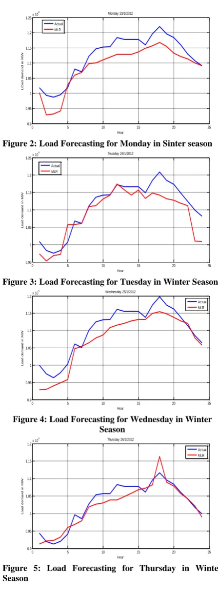
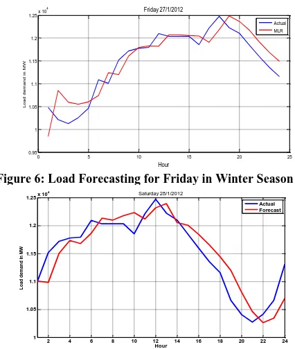
5.1 Winter Model

The method of MLR was applied to predict the load for each day in the forecasted week, which covering the period from January 22, 2012 till January 28, 2012 for winter season. The real data for Iraqi network will be taken from Iraq operation and control center which represents the actual daily load for the winter (January) season of the year 2012.

Figures from (1) to (7) show the actual and the forecasted load for each day in the forecasted week for winter season.

0 5 10 15 20 25

1 1.05 1.1 1.15 1.2 1.25 1.3x 10

4 _{Sunday 22/1/2012}

Hour

L

o

a

d

d

e

m

a

n

d

i

n

M

W

Actual MLR

Figure 1: Load Forecasting for Sunday in Winter Season

0 5 10 15 20 25

0.9 0.95 1 1.05 1.1 1.15 1.2 1.25x 10

4 _{Monday 23/1/2012}

Hour

L

O

a

d

d

e

m

a

n

d

i

n

M

W

Actual MLR

Figure 2: Load Forecasting for Monday in Sinter season

0 5 10 15 20 25

0.95 1 1.05 1.1 1.15 1.2 1.25x 10

4 _{Teusday 24/1/2012}

Hour

L

o

a

d

d

e

m

a

n

d

i

n

M

W

Actual MLR

Figure 3: Load Forecasting for Tuesday in Winter Season

0 5 10 15 20 25

0.9 0.95 1 1.05 1.1 1.15 1.2x 10

4 _{Wednesday 25/1/2012}

Hour

L

o

a

d

d

e

m

a

n

d

i

n

M

W

Actual MLR

Figure 4: Load Forecasting for Wednesday in Winter Season

0 5 10 15 20 25

0.9 0.95 1 1.05 1.1 1.15 1.2x 10

4 _{Thursday 26/1/2012}

Hour

L

o

a

d

d

e

m

a

n

d

i

n

M

W

Actual MLR

0 5 10 15 20 25 0.95 1 1.05 1.1 1.15 1.2 1.25x 10

4 Friday 27/1/2012

Hour L o a d d e m a n d i n M W Actual MLR

Figure 6: Load Forecasting for Friday in Winter Season

2 4 6 8 10 12 14 16 18 20 22 24

1 1.05 1.1 1.15 1.2 1.25x 10

4 Hour L o a d d e m a n d in M W Saturday 28/1/2012 Actual Forecast

Figure 7: Load Forecasting for Saturday in Winter Season

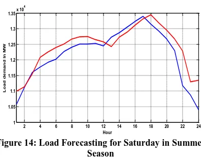
5.2 Summer Model

The method of MLR was applied to predict the load for each day in the forecasted week, which covering the period from June 22, 2012 till June 28, 2012 for summer season.

Figures from (8) to (14) show the actual and the forecasted load for each day in the forecasted week for summer season.

0 5 10 15 20 25

1 1.05 1.1 1.15 1.2 1.25 1.3 1.35 1.4 1.45 1.5x 10

4 _{Sunday 22/7/2012}

Hour L o a d d e m a n d i n M W Actual MLR

Figure 8: Load Forecasting for Sunday in Summer Season

0 5 10 15 20 25

1.1 1.15 1.2 1.25 1.3 1.35 1.4 1.45 1.5 1.55x 10

4 _{Monday 23/7/2012}

Hour L o a d d e m a n d i n M W Actual MLR

Figure 9: Load Forecasting for Monday in Summer

2 4 6 8 10 12 14 16 18 20 22 24

1.1 1.15 1.2 1.25 1.3 1.35 1.4 1.45 1.5 1.55x 10

4 Hour F o re c a s t lo a d i n M W Tuesday 24/7/2012 Actual MLR

Figure 10: Load Forecasting for Tuesday in Summer Season

2 4 6 8 10 12 14 16 18 20 22 24

1.1 1.15 1.2 1.25 1.3 1.35 1.4 1.45 1.5 1.55x 10

4 Hour lo a d d e m a n d i n M W Wednesday 25/7/2012 Actual MLR

Figure 11: Load Forecasting for Wednesday in Summer Season

2 4 6 8 10 12 14 16 18 20 22 24

1.05 1.1 1.15 1.2 1.25 1.3 1.35

1.4x 10 4 Hour L o a d d e m a n d i n M W Actual MLR

Figure 12: Load Forecasting for Thursday in Summer Season

2 4 6 8 10 12 14 16 18 20 22 24

1.1 1.15 1.2 1.25 1.3 1.35 1.4 1.45

1.5x 10 4 Hour lo a d d e m a n d i n M W Friday 27/7/2012 Actual MLR

Volume 100– No.1, August 2014

2 4 6 8 10 12 14 16 18 20 22 24

1 1.05 1.1 1.15 1.2 1.25 1.3 1.35x 10

4

Hour

L

o

a

d

d

e

m

a

n

d

i

n

M

W

Figure 14: Load Forecasting for Saturday in Summer Season

The MAPE index can be used as an estimation of the goodness of the fit for the models, Table (1) provide a summary of those MAPE values.

Table 1: MAPE of Winter and Summer Seasons for MLR Method

DAY

Winter Model

Summer Model

Sunday 1.604 2.083 Monday 2.963 1.244 Tuesday 2.0179 1.89 Wednesday 2.475 1.87 Thursday 0.7146 1.121

Friday 1.01 1.867 Saturday 1.91 1.774

6. CONCLUSION

The problem for forecasting the demand load power for Iraq is a typical and intricate which makes such a problem a challenge and perhaps unique in its nature. This stems from the fact that there are many complex factors that influence the amount of load needed each season. Some of these factors are:

 The rapid economical, commercial, and population growth of the country.

 The large diversity of minimum and maximum temperatures over seasons: typically, the high temperature period (July and August) is characterized by

high ambient temperatures that may exceed 47

o

C and the minimum can drop to subzero degrees in winter. The result of load forecasting contains several components of errors, namely, modeling error (error introduced to regression), error caused by system disturbances such as load

shedding and irregular events and also errors of temperature forecast. This model is very sensitive to the fluctuation of temperature. It needs a very accurate temperature forecast, as a small change of temperature will cause a significant change in load prediction.

7. REFERENCES

[1] J. P. Rothe, A. K. Wadhwani and S. Wadhwani, “Short Term Load Forecasting Using Multi Parameter Regression”, International Journal of Computer Science and Information Security (IJCSIS), Vol. 6, No. 2, 2009.

[2] S.A. Soliman, and A.M. Al-Kandari, “Electrical Load Forecasting: Modeling and Model Construction”, pp. 82-93, 2010.

[3] S.A.Soliman, S. Persaud, K. Nagar and M.E. El-Hawary, “Application of Least Absolute Value Parameter Estimation Technique Based on Linear Programming to Short-Term Load Forecasting”, IEEE, pp. 529-533, 1996.

[4] Hesham K. Alfares and Mohammad Nazeeruddin, “Electric load forecasting: literature survey and classication of methods”, International Journal of Systems Science, volume 33, No.1, PP. 23±34, 2002.

[5] Nahid-Al-Masood, Mehdi Z. Sadi, Shohana Rahman Deeba and Radwanul H. Siddique, “Temperature Sensitivity Forecasting of Electrical Load”, The 4th International Power Engineering and Optimization Conf. (PEOCO), PP. 23-24, MALAYSIA, June 2010.

[6] Nazih Abu-Shikhah, Fawwaz Elkarmi and Osama M. Aloquili, “ Medium-Term Electric Load Forecasting Using Multivariable Linear and Non-Linear Regression ”, Smart Grid and Renewable Energy, PP. 126-135, Vol. 2, 2011.

[7] J. P. Rothe, A. K. Wadhwani and A. K. Wadhwani, “Hybrid and Integrated Approach to Short Term Load Forecasting”, International Journal of Engineering Science and Technology Vol. 2(12), PP.7127-7132, 2010.

[8] M. Babita Jain, Manoj Kumar Nigam and Prem Chand Tiwari, “A Parameter based New Approach for Short Term Load Forecasting using Curve-fitting and Regression line method”, International Journal of Engineering Research & Technology (IJERT) Vol. 1, August – 2012.