ID3 Modification and Implementation in Data Mining

(1)

ID3 Modification and Implementation in Data Mining

Hemlata Chahal

Lecturer, Technical Education Department, Panchkula,

Haryana

ABSTRACT

In this paper, ID3 algorithm of decision trees is modified due to some shortcomings. The algorithm is implemented to create a decision tree for bank loan seekers.ID3 algorithm is an existing algorithm which is modified because the dataset cannot be implemented in the existing conditions. Some changes are done in order to remove the shortcomings of the algorithm. Now the modified version is implemented in the dataset taken. With the help of the modified algorithm a decision tree is created which is helpful to the bankers to predict the credit risk of the loan seekers from the bank.

Keywords

Decision Tree, Iterative Dichotomiser 3 algorithm, Entropy, Information Gain.

1. INTRODUCTION

In today’s world, the organizations strive for neck to neck competition. To exist in the market every organization has to take correct and efficient decisions. So decision making activity is the most important activity for the businessmen. They have to analyze all the existing data and conditions for decision making. They have to extract new information out of the new existing information. Only because of this new information the decision makers can take competitive decisions.

The technique to extract new knowledge form the existing information is known as data mining. There are different techniques to mine the data from databases. One important technique is classification and segmentation, under which decision trees are created in order to predict the data from the existing one. Decision trees are created with the help of different algorithms. One such algorithm, namely, ID3 is used here.

2. DATA MINING

Data mining, the extraction of hidden predictive information from large databases, is a powerful new technology with great potential to help companies focus on the most important information in their data warehouses. [1]

3. DECISION TREES

Decision tree is powerful and popular tool for classification and prediction. Decision trees represent rules. A decision tree is predictive model that, as its name implies, can be viewed as a tree. Specifically each branch of the tree is a classification question and the leaves of the tree are partitions of the dataset with their classification. [4]

Decision tree is a classifier in the form of a tree structure, where each node is either:

 a leaf node- indicates the value of the target

attribute(class) of examples, or

 a decision node- specifies some test to be carried out on a single attribute- value, with one branch and sub-tree for each possible outcome of the test.

3.1 Constructing Decision Trees [6]

Most algorithms that have been developed for learning decision trees are variations on a core algorithm that employs a top-down, greedy search through the space of possible decision trees. Decision tree programs construct a decision tree T from a set of training cases.

4. DECISION TREE ALGORITHM:

The decision tree algorithm creates hierarchical structure of classification rules “If-Then” looking like a tree. Much work has been done in the field of decision tree algorithm [2].

J.Ross Quinlan originally developed ID3 algorithm at the University of Sydney. He first presented ID3 in 1975 in a book “Machine Learning”, vol.1, no.1. ID3 is based on the concept Learning System algorithm[3].

5. ID3 ALGORITHM [3]

Iterative Dichotomiser 3 is an algorithm used to generate a decision tree. The algorithm is based on Occam’s razor: it prefers smaller decision trees over larger ones. However, it does not always produce the smallest tree, and therefore a heuristic.

5.1 ID3 (Examples, Target_Attribute,

Attributes)

 Create a root node for the tree.

 If all examples are positive, Return the single-node tree Root, with label = +.

 If all examples are negative, Return the single-node tree Root, with label = -.

 If number of predicting attributes is empty, then Return the single node tree Root, with label= most common value of the target attribute.

 Otherwise Begin

 A= The Attribute that best classifies examples.  Decision Tree attribute for Root = A

 For each possible value, vi, of A,

 Add a new Tree branch below Root,

corresponding to the test A = vi.

 Let Examples(vi), be the subset of examples

(2)

 If Examples (vi) is empty, then below this new

branch add a leaf node with label = most common target value in the examples.  Else below this branch add the subtree ID3 (

Examples(vi), Target_Attribute, Attributes-{A})  End

 Return Root

ID3 searches through the attributes of the training instances and extracts the attribute that best separates the given examples. If the attribute perfectly classifies the training sets then ID3 stops; otherwise it recursively operates on the m (where m=number of possible values of an attribute) partitioned subsets to get their “best” attribute. The algorithm uses a greedy search, that is, it picks the best attribute and never looks back to reconsider earlier choices.

The central focus of the decision tree growing algorithm is selecting which attribute with the most inhomogeneous class distribution the algorithm uses the concept of entropy.

5.2 Information Entropy [4]

Entropy(S) is a measure of how random the class distribution is in S.

Entropy(S) = - pplog2pp - pnlog2pn

Where pp is the proportion of positive examples in S and pn is

the proportion of negative examples in S.

Information Gain measures how well a given attribute separates the training examples according to their target classification.

Gain(S,A) = Entropy(S)-

6. MODIFIED ID3 ALGORITHM:

In ID3 Algorithm, every attribute has the binary valued domain (i.e. positive or negative). But it is also possible that we have some specific attributes that have multiple valued domain (i.e. high, medium, low, etc.). For such attributes the algorithm can be modified as below:-

6.1 Modified ID3 (Examples,

Target_Attribute, Attributes)

 Create a root node for the tree.

 If all examples are of same value say high, medium, low..., Return the single-node tree Root, with label = High, Medium, Low,...

 If number of predicting attributes is empty, then Return the single node tree Root, with label= most common value of the target attribute.

 Otherwise Begin

 A= The Attribute that best classifies examples or in other words the attribute with highest information gain value.

 Decision Tree attribute for Root = A  For each possible value, ai, of A,

 Add a new Tree branch below Root,

corresponding to the test A = ai.

 Let Examples(ai), be the subset of examples

that have the value ai for A.

 If Examples(ai) is empty, then below this new

branch add a leaf node with label = most common target value in the examples.

 Else below this new branch add the subtree ID3

( Examples(ai), Target_Attribute,

Attributes-{A})  End

 Return Root

___

7. IMPLEMENTATION OF THE

MODIFIED ID3 ALGORITHM

7.1 About the Dataset Taken

The data set was taken from a national bank which consisted of the loan customers. In the bank a Performa of the loan seekers is being filled to calculate the credit risk. Many attributes are taken into account for the calculation of credit risk. After calculating the credit risk, decision is taken from the following three options:-

 Accepting loan application without guarantor.

 Accepting loan application with guarantor.

 Rejecting loan application.

All the attributes were generalized into 8 important attributes (Age, Educational Qualification, Marital Status, No. of

dependents, Employer/Profession, Years in current

employment, Net Annul Income, No. of years having a/c with the bank) for the calculation of credit risk. The data is represented in the table 6.1.

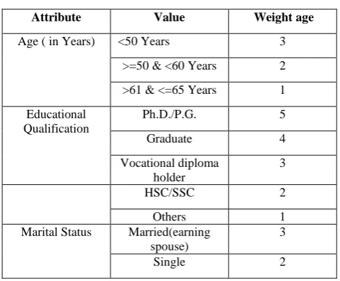
[image:2.595.307.552.558.760.2]

The credit risk is the Target Attribute (also called the class attribute). The target attribute (i.e. credit risk) has the domain as {High, Medium, Low} based on the values of other attributes. The value of credit risk is predicted according to the weight age given to other attributes. The domain and weight age of all the attributes is given below:

Table 7.1: Loan Score Card

Attribute Value Weight age

Age ( in Years) <50 Years 3

>=50 & <60 Years 2

>61 & <=65 Years 1

Educational Qualification

Ph.D./P.G. 5

Graduate 4

Vocational diploma holder

3

HSC/SSC 2

Others 1

Marital Status Married(earning

spouse)

3

(3)

Married(non-earning spouse)

1

No. of dependents 0-1 5

2 4

3 3

4 2

>=5 1

Employer/Professi on

MNC/Central Govt./Doctor/Comp

uter

10

Professional/ Engineer/ Architect Reputed Public Ltd.

Co./C.A.

8

State Govt./ Lawyer/ Artist/

Professional Sportsman/ Agriculturist/

Contractor

6

Local civic bodies/ Pvt. Co./ Firms

4

Others 2

Years in current profession

>=8 5

>=6 4

>=4 3

>=2 2

<2 1

Net Annual Income(NAI)

>=6 lacs 5

>=4 & <6 lacs 4

>=2.5 & <4 lacs 3

>=1 & <2.5 lacs 2

<1 lac 1

No. of years having a/c with

the bank

>=5 years 4

>=3 & <5 years 3

>=2 & <3 years 2

[image:3.595.46.549.68.469.2]

>=1 & <2 years 1

Table 7.2: Decision about Loan Target

Attribute

Domain Total Weight age Of Other Attributes

Decision

Credit Risk

Low >32 The loan will be

given without Guarantor

Medium 27-31 The loan will be

given with Guarantor

High <27 The loan cannot

[image:3.595.49.574.504.768.2]

be given.

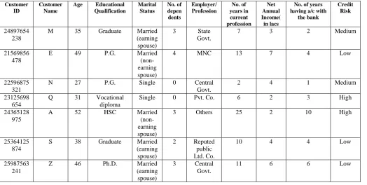
Table 7.3: Dataset of existing customers

Customer ID

Customer Name

Age Educational Qualification

Marital Status

No. of depen

dents

Employer/ Profession

No. of years in current profession

Net Annual Income( in lacs

No. of years having a/c with

the bank

Credit Risk

24897654 238

M 35 Graduate Married

(earning spouse)

3 State

Govt.

7 3 2 Medium

21569856 478

E 49 P.G. Married

(non-earning spouse)

4 MNC 13 7 4 Low

22596875 321

N 27 P.G. Single 0 Central

Govt.

2 4 1 Medium

23125698 654

Q 31 Vocational

diploma

Single 0 Pvt. Co. 6 2 3 High

24365128 975

A 52 HSC Married

3 Others 25 2 10 High

25364125 874

S 38 Graduate Married

(earning spouse)

2 Reputed

public Ltd. Co.

10 4 4 Low

25987563 241

Z 46 Ph.D. Married

(earning spouse)

3 Central

Govt.

(4)

26564231 256

X 30 Others Married

2 Pvt. Firms 5 2 3 High

26897565 231

F 42 Vocational

diploma

Married (non-earning spouse)

2 State

Govt.7

8 3 7 Medium

27589654 236

B 48 Graduate Married

(earning spouse)

3 Reputed

Public Ltd. Co.

12 4 10 Low

27985641 236

V 29 P.G. Single 1 MNC 3 5 2 Low

29856475 623

C 38 P.G. Married

(earning spouse)

2 Reputed

Public Ltd. Co.

6 5 5 Low

30025469 875

L 29 P.G. Married

(earning spouse)

2 C.A. 3 4 2 Medium

31026589 745

K 34 Ph.D. Married

(earning spouse)

3 State

Govt.

5 6 4 Medium

32156234 698

J 46 Graduate Married

4 Lawyer 6 7 4 Medium

33265498 745

H 51 HCS Married

5 Agricultur

ist

18 3 10 High

33896547 895

G 36 Vocational

Diploma

Married (non-earning spouse)

3 Contractor 11 3 5 Medium

34562159 875

F 49 Graduate Married

4 Engineer 19 8 10 Low

34652315 462

D 28 Graduate Single 1 Doctor 1 6 1 Medium

35642398 756

S 30 Others Single 2 Others 2 2 2 High

35564851 236

R 42 SSC Married

2 Profession

al Sportsman

18 6 10 Medium

36025412 365

T 37 P.G. Married

(earning spouse)

2 Computer

Profession al

12 8 5 Low

37654239 546

Y 32 Vocational

diploma

Married (earning

spouse)

3 Contractor 6 4 4 Medium

37023654 128

U 39 PhD Married

(earning spouse)

2 Central

Govt.

12 6 10 Low

37236547 896

I 29 Graduate Single 2 Architect 3 5 3 Low

37778954 623

O 50 P.G. Married

4 Computer

profession al

(5)

7.2 Calculation of Entropy and

Information Gain

For implementing the modified ID3 algorithm, the information Gain and Entropy is calculated as follows-:

Entropy(S) = Entropy (11L, 10M, 5H) = -(11/26)*log2(11/26) -

(10/26)*log2(10/26)

-(5/26)*log2(5/26)

= -11/26(-1024101)- 10/26(-1.37851) - 5/26(-2.37851)

= 1.512645

= 1.512645-(23/26)*Entropy(S3) -

(3/26)*Entropy(S2)-

(0/26)*Entropy(S1)

= 1.512645-(23/26)*[-(3/23)*

log2(3/23)-(10/23)*log2(10/23)-

(10/23)*log2

(10/23)]-(3/26)*[- (2/3)log2(2/3)-(0/3)log2(0/3)-(1/3)log2(1/3)]-0

= 1.512645-(23/26)*1.428195-(3/26)*0.918296-0

= 0.143285

Similarly other Gain values can also be calculated and their values are as follows:-

Gain(S, E.Q.)= 0.677664 Gain(S, Marital Status)= 0.16923 Gain(S, No. of dep.)= 0.258564 Gain(S, Profession) = 0.984468 Gain(S, No. of Years) = 0.374909 Gain(S, NAI) = 0.370136 Gain(S, Years of a/c) = 0.144817

Having the gain value as above, a decision tree can be drawn with first attribute having the highest gain value i.e. Profession ( gain value= 0.984468). Next attribute taken is

Educational Qualifications(gain value= 0.677664). And so on....

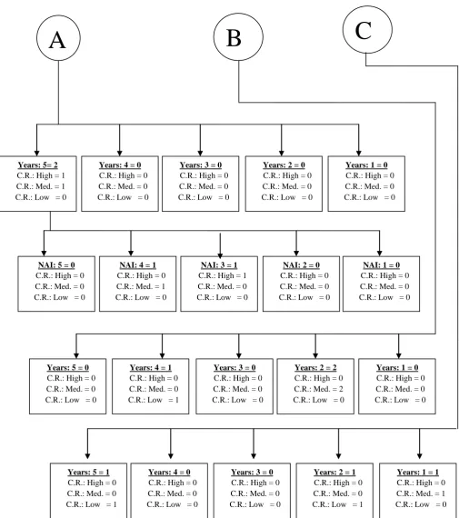
7.3 Creation of decision Tree

(6)

jjjj

All Cases

Credit Risk: High = 5 Credit Risk: Medium = 10 Credit Risk: Low = 11

Prof.: 2 = 1

C.R.: High = 1 C.R.: Med. = 0 C.R.: Low = 0

Prof.: 4 = 3

C.R.: High = 3 C.R.: Med. = 0 C.R.: Low =

0

Prof.: 6 = 8

C.R.: High = 1 C.R.: Med. = 7 C.R.: Low =

0

Prof.: 8 = 5

Prof.: 10 = 9

E.Q.: 4 = 2

E.Q.: 5 = 1

E.Q.: 2 = 2

E.Q.: 1 = 0

E.Q.: 3 = 3

E.Q.: 3 = 0

E.Q.: 4 = 2

E.Q.: 5 = 3

E.Q.: 2 = 0

E.Q.: 1 = 0

E.Q.: 5 = 6

E.Q.: 4 = 3

E.Q.: 3 = 0

E.Q.: 2 = 0

E.Q.: 1 = 0

C

B

(7)

[image:7.595.51.557.74.645.2]

Figure 7.1: Decision Tree Years: 5= 2

A

B

C

Years: 4 = 0

Years: 1 = 0

Years: 3 = 0

Years: 2 = 0

NAI: 5 = 0

NAI: 4 = 1

NAI: 3 = 1

NAI: 2 = 0

NAI: 1 = 0

Years: 2 = 2

Years: 3 = 0

Years: 4 = 1

Years: 5 = 0

Years: 1 = 0

Years: 5 = 1

Years: 4 = 0

Years: 3 = 0

Years: 2 = 1

Years: 1 = 1

(8)

7.4 Interpretation of decision tree

The above decision tree is beneficial in the situation where a new customer approaches the bank for loan. The bank first of all checks the profession of the customer.

If the profession comes in the category with grade as 4 or 2, directly from the decision tree it can be seen that his credit risk is very high, so the customer is rejected a loan. If the profession falls in the category with grading 6, his educational qualification is checked and if the grading of E.Q. is 5, 4 or 3 the credit risk is found to be Medium i.e. the customer is provided the loan but with a guarantor. If the grading of E.Q. is 2, the number of years of the current profession of the customer is checked. The grading of number of years is checked, if it comes out to be 2, the his Net Annual Income(including spouse’s income) is to be calculated and if it also falls in the category with grade 4, then Credit Risk is Medium. The customer is given the loan with a guarantor. But if NAI grade is 3, credit risk is high and the customer is rejected the loan. If the grading of profession the customer is 8, his Educational Qualification is calculated and the grade of E.Q. is 4, the Credit Risk is low and the customer is provided the loan without guarantor.

Hence by traversing the tree the bankers can take the decision about loan to the customers.

8. SCOPE FOR FUTURE WORK

In this work a decision tree is created for the bankers that will be useful to predict the status of the credit risk of loan seeker customers by considering eight parameters or attributes. But

the bank considers more than 20 parameters to calculate the credit risk. So, there is a scope to extend the study by considering all of the attributes. The decision tree can created using any other commercial algorithm. Also the open issues for the researchers can be efficiency of the tree i.e. reduction of complexity, reduction of depth of the tree etc.

9. REFERENCES

[1] Kurt Thearling, “An Introduction to Data Mining”, a paper published in “Data Mining-Vol-1”, ICFAI [2002].

[2] http://www.bandmservices.com/DecisionTrees/Decision

_trees.htm

[3] Quinlan, J.R. [1986], Introduction of decision trees, “Machine Learning”.

[4] H.Hamilton. E. Gurak, L. Findlater W. Olive, “Overview

of Decision Trees” as published on the website http://www.cs.uregina.cd/~dbd/cs831/notes/ml/dtrees/4_ dtrees1.html

[5] http://en.wikipedia.org/wiki.ID3_algorithm#algorithm

[6] Nagabhushana, S., [2006] “Data Warehousing-OLAP

and Data Mining”, New Age International Publishers. [7] Chaudhari, S., and Dayal, U. [1997] “An Overview of

Data Warehousing and OLAP Technology”,SIGMOD Record, Vol.26, No. 1, March 1997.

[8] Breiman,L., Friedman,J.H., Olsen,R.A., and

Stone,C.J.(1984) “Classification and Regression