Techniques of Binarization, Thinning and Feature Extraction Applied to a Fingerprint System

Techniques of Binarization, Thinning and Feature

Extraction Applied to a Fingerprint System

Romulo Ferrer L. Carneiro

Instituto Federal do Ceara

Jessyca Almeida Bessa

Instituto Federal do Ceara

Jermana Lopes de Moraes

Instituto Federal do Ceara

Edson Cavalcanti Neto

Universidade Federal do Ceara

Auzuir Ripardo de Alexandria

Instituto Federal do Ceara

ABSTRACT

A large volume of images of fingerprints are collected and stored to be used in various systems such as in access control and iden-tification records (ID). Systems for automatic fingerprint recogni-tion perform searches and comparisons with a database. Biometric recognition is based on two fundamental premises: the first is that digital printing must have permanent details, and the second is the information unit. From these premises, a system analyzes the fin-gerprint image to extract the information and then compares the data in the verification mode or identification mode. , Extraction techniques must be used to obtain the fingerprint data. These tech-niques use binarization, thinning and features extraction algorithms which are computational methods that can be applied to digital im-age processing used in scientific research and security issues. This paper presents a comparative analysis of four thresholding tech-niques (Niblack, Bernsen, Fisher, Fuzzy), two thinning techtech-niques (Stentiford and Holt) and a feature extraction (Cross Number) tech-nique to evaluate the best performance of the algorithms in finger-print images. To develop this project a set of 160 fingerfinger-print images was used in experiments and analysis. The results point out the pos-itive and negative points of the different algorithms. The system was developed in the C/C++ language.

Keywords:

Images of fingerprints, Thresholding, Thinning, Feature Extraction.

1. INTRODUCTION

Nowadays, there are a number of biometric systems available and they are being used more and more for almost everything that needs security or identification and verification. Biometric recognition, or simply biometrics, refers to the use of distinctive anatomical and behavioral characteristics or identifiers (e.g., fingerprints, face, iris, voice, hand geometry) for automatically recognizing a person. Be-cause of the well-known distinctiveness (individuality) and persis-tent properties of fingerprints as well as the low cost of the devices to capture the images, fingerprints have become the most widely used biometric characteristic. It is generally believed that the pat-tern on each finger is unique [8]. Consequently, fingerprints have emerged as the most common and trusted biometric for personal identification. Fingerprints were first introduced as a method for person identification over 100 years ago. Nowadays, every

foren-Fig. 1: 3-D representation of the structure of skin [6].

sics and law enforcement agency worldwide routinely uses au-tomatic fingerprint identification systems (AFIS)[10]. Fingerprint recognition systems can be viewed as pattern recognition systems. Fingerprint matching involves an input of some fingerprint images and the output is the probability that the fingerprints are from the same finger. So fingerprint identification technology basically car-ries out four functions: reading the fingerprint, feature extraction, saving the data and comparison. This paper presents improved al-gorithms for fingerprint image recognition; it presents a compara-tive analysis of four techniques of thresholding (Niblack, Bernsen, Fisher, Fuzzy) and two thinning techniques (Stentiford and Holt) that allow a reduction in the computational cost of the recognition system [15]. Also a feature extraction method (Cross Number) was implemented to evaluate the algorithms performance in fingerprint images. The paper is organized into five parts: Section 2 brings a brief overview of the biometric system. Section 3 presents the tech-niques of digital image processing applied to fingerprints. Section 4 describes a comparative analysis of implemented algorithms and Section 5 gives the conclusions of this work.

2. BIOMETRIC SYSTEM

Fig. 2: singular regions (rectangles) and reference points (solid circles)[10] .

Fig. 3: five main types of fingerprint classification as defined by Henry a) left loop; b) right loop; c) vertical; d) ark; e) tent ark [4].

Fingerprint analysis for matching purposes generally requires the comparison of several features of the print pattern. These include patterns, which are aggregate characteristics of ridges, and minu-tia points, which are unique features found within the patterns. It is also necessary to understand the structure and properties of hu-man skin in order to successfully apply some of the imaging tech-nologies [12]. A typical fingerprint analysis system is based on monochrome image analysis and it is made up of two steps. The first step can be in four stages: scanning images (acquisition), seg-mentation (binarization), skeletonization (thinning) and feature ex-traction (minutiae); and this is generally carried out in a sequential manner [7]. The second step is the recognition process itself; how-ever it is not the aim of this work to go into detail on this point. Fin-gerprints have different ratings as the formats defined by the ridges and valleys. These formats can be classified into three topologies: Loop, Whorl and Delta, as shown in Figure 2.

Fingerprint images have a central point called the nucleus which determines the classification of the image. However, the singular-ities of these central points hinder its classification. However, it is possible to classify them according to natural regions [4], and there-fore they can be analyzed as shown in Figure 3.

Most fingerprint recognition systems use minutiae extraction tech-niques for verifying comparisons [13]. The techtech-niques to extract minutiae evaluate the different forms of ridges present in a finger-print. What defines the uniqueness of a person is present in each set of fingerprint minutiae. The types of minutiae are shown in Figure 4.

It is important to know the difference between verification and identification in a biometric system. These are applied in finger-print recognition systems and so the user must understand the three stages of fingerprint recognition: registration, verification and iden-tification. Assuming that the user has performed the registration of the sample (template) in the database, the registration steps are out-lined in Figure 5.

The maximum extraction of minutiae is very important for finger-print recognition systems. However, this step can only be carried out after the completion of the two preceding stages, which im-prove the image greatly, facilitating the detection of the minutiae.

Fig. 4: Types of minutiae [7]).

Fig. 5: Block diagram of Registration [10].

3. TECHNIQUES OF DIGITAL IMAGE

PROCESSING APPLIED TO FINGERPRINTS

The information must be computationally processed in a format suitable for processing the scanned image. A digital image is repre-sented by a matrix with rows and columns which identify a point in the image functionf(x, y)called a pixel [3]. A monochrome image is represented by a two-dimensional mathematical functionf(x, y)

whose value indicates the intensity at point(x, y). This function is the result of the product of illuminationi(x, y)by the reflectance

r(x, y), wherei(x, y)indicates the amount of light striking the ob-ject, andr(x, y)indicates the amount of light reflected by the ob-ject, as can be seen in Equation 1.

f(x, y) =i(x, y)·r(x, y);

where0 < i(x, y) < ∞; (1)

e0 < r(x, y) < 1;

According to this information, a fingerprint image captured by a fingerprint sensor is stored in a digital format that is subsequently processed and visualized. After binarization, the fingerprint images have black points with a value of zero (0) and white points with a value of one (1).

Fig. 6: Pixel neighborhood. a) neighborhood of 4 pixels; b) neighborhood of 8 pixels.

To evaluate the position of the pixels a pointP(x, y)is defined as the central point and the movement of its adjacent points clockwise. Then an imaginary plane is drawn over the center point, so that the coordinate is x and the ordinate is y. The connectivity between the pixels is defined by an analysis of the adjacent points that have the same properties as the central pixel P using a mask with a 4 or 8 neighborhood.

3.1 Segmentation by thresholding

Segmentation by thresholding is a technique of segmenting the more popular regions due to its simplicity and low use of processing memory; however the great difficulty lies in choosing the threshold so that the information of interest is extracted from the image with perfection [11].

Segmentation aims to analyze an image in order to extract the at-tributes or characteristics of interest. The extraction of information is based on the discontinuity (contours) or the similarity (regions) of the properties of the values of the gray levels in an image. [3] Thresholding is one of the most important methods in the image segmentation. Its goal is to separate the foreground of the object (area of interest) from the background by comparing the value of gray level of each pixel pointpinf(x, y)with a thresholdL. The threshold valueLis a gray level so that the pixels whose lumi-nous intensity is larger thanLbelong to the region of interest and the remaining pixels belong to the background. The equation which defines the threshold (GONZALEZ; WOODS, 2002) is given equa-tion 2.

g(x) =

1, if f(x, y)> L

0, otherwise (2)

where f (x, y) is the result of the thresholding process of each point, and L is a value chosen to separate the foreground from the back-ground; the threshold value can be chosen automatically or manu-ally.

3.1.1 Global thresholding. When the goal is a single threshold value for the entire image, the process is said to be global thresh-olding. The automatic choice of this threshold value can be done by analyzing a histogram of the image.

3.1.2 Adaptive local thresholding. Due to the complexity of se-lecting a global threshold, another way to define binarization is based on the analysis of the intensities of gray levels within a local window over an image, so that local thresholds can be determined.

3.2 Evaluation of thresholding algorithms

The algorithms evaluated in this paper are based on two types of thresholding: the local adaptive algorithms that include Niblack

[11], Bernsen [1] and the global algorithm which includes the Fisher [9] and Fuzzy Dens algorithms [15].

3.2.1 Adaptive thresholding by Bernsen. The adaptive threshold-ing by Bernsen calculates the gray level values present in each pixel P (x, y) neighborhood to obtain the threshold value of each pixel (x, y) using equation 3.

P(x, y) =(P highest−P lowest)

2 (3)

where Plowest and Phighest are the lowest and highest values of gray level present in the square neighborhood of R x R centered at pixel (x, y). The contrast of the gray levels can be calculated by Equation 4.

C(x, y) = (P highest−P lowest) (4) where C (x, y) is the value of the contrast and (Phighest-Plowet) is smaller than a value L value, which is the minimum contrast, so thus the neighborhood is said to be belonging to the same region of homogeneous pixels or better a partition of pixels.

3.2.2 Adaptive thresholding by Niblack. Niblack’s thresholding algorithm is an adaptive local thresholding method based on a sta-tistical analysis between each pixel and its neighborhood [11]. This algorithm is based on the calculation of the mean (µ) and stan-dard deviation (s) of the neighborhood around each image pixel to be binarized [2].

The value of the mean (µ) is given by equation 5.

µ(x, y) = 1

N.M

N

X

x=0 M

X

y=0

p(x, y) (5)

The standard deviation (s) of the neighborhood around each image pixel is calculated by Equation 6.

s(x, y) = r

1

N.M

N

X

x=0 M

X

y=0

(p(x, y)−s(x, y))2 (6)

To calculate the threshold (L) of each pixel is calculated using equa-tion 7.

L(x, y) =−α.s(x, y) +s(x, y) (7) The Fisher thresholding consists in optimizing of P partitions or groupings of thresholds through using the a dynamic type of algo-rithm [9]. LetW = [0, ..., L−1]the set of gray levels of the image and P = (C1, C2, ... CN) a partition of W in Nc classes in gray lev-els. Consider k as the index of the current gray level,h(k)the num-ber of pixels of the gray level k, and c a counter of c classes gray. The optimum criterion of the Fisher method consists in minimizing the sum of the inertia of the Nc cluster Nc. We use the equation 8 and 9 to find an inertiaW(P)associated with a partition use the equations 8 and 9.

W(P) =

N c

X

n=1

X

keCn

h(k).(k−G(Cn))2 ₍₈₎

G(Cn) = P

KeCnK.h(k)

P

KeCnh(k)

whereG(Cn) represents the center of gravity of class Nc for a given subset ofW. To find the is its inertia ofW useing equations 10 and 11.

Gab= Pb

k=ak.h(k)

Pb

k=ah(k)

(10)

Iab=

b

X

k=a

h(k).(k−Gab) (11)

whereIabdenotes the inertia associated with an intervalab. In the particular case of a segmentation which involves only two classes of gray levels, one can find the threshold can be found between the two classes C1 and C2 in order to minimize the inertiaW(P), adapting the formulas used for the general case n-classes of the grayscale to only two classes [9]. According to equation 12.

W(P) = X

keC1

h(k).(k−G(Cn))2₊X keC2

h(k).(k−G(C2))2 (12) Optimizing Equation 12, its minimization becomes the maximiza-tion of equamaximiza-tion 13.

J(P) = ( P

k=C1k.h(k)) 2

P

k=C1h(k)

+( P

k=C2k.h(k)) 2

P

k=C2h(k)

(13)

The problem is to find a level a belonging to the range of gray levels

[0, L−1]such thatJ(P)is the maximum [9].

3.2.3 Fuzzy thresholding through estimation of normal densities. The algorithm for estimating normal densities works with the nor-mal distribution of the gray levels of the object and the background [15]. A thresholding strategy is based on equation 14.

j(T) =

T−1

X

j=0

pj{(j−v1

s1 )

2_{+ 2.log s1−pj}}

(14)

+ PL−1 j=Tpj{(

j−v2 s2 )

2_{+ 2.log s2−pj}}

9wherev1is the average grayscale of the object (between 0 and T -1);v2is the average grayscale of the background (between T and 255);s1is the standard deviation of the grayscale of the object;

s2is the standard deviation of the grayscale of the background and pj is the normalized histogram relative to the amount of pixels The global minimum ofJ(T)is the appropriate threshold for separating the object from the background. The absolute threshold is defined by using a distance measurement associated with each class. For this purpose, pseudo distance functions are defined according to equation 15.

d(j, vi) =1 2(

j−vi si )

2

+log si−logβ i (15) Whereβiandsiare given by equations 16 e and 17.

β1 =

PL−1

j=0µ(j).hj

PL−1

j=0µ0(j).h1 +

PL−1

j=0µB(j).hj

(16)

si= PL−1

j=0µi(j).hj.(j−vi) 2

PL−1

j=0µi(j).hj

(17)

Fig. 7: neighborhood structure used in thinning algorithms.

whereµis the pertinence function of each gray level to one of the classes (background and or object).

The problem of fuzzy clustering consists in the partitioning of n sampling points in c classes in which membership functions have the properties of the equations 18, 19 and 20.

µi(xj)ε[1,0] (18)

0>

n

X

j=1

µi(xj)< n (19)

c

X

i=1

µi(xj) = 1,0 (20)

The fuzzy thresholding method of thresholding algorithm, using fuzzy estimates of normal densities, may be described in the fol-lowing steps:

(1) Initialize the threshold descriptorµoandµb, which satisfy the equations 18,19 and 20

(2) Compute the median values of both regions using equation 21.

vi= PL−1

j=0hj.j.µi(j) T

PL−1

j=0hj.µi.(j)

T (21)

(3) Computeβi andsi , using the Equations 16 and 17, respec-tively;

(4) Improve the members using Equation 22.

µo(j) =

1

1 + [_dd₍(_j,vb,vo)₎]· 2 (T−1)

(22)

(5) Repeat steps 2-5 until there are no more changes inµ0andµb .

3.3 Image thinning process

The thinning technique is often used to get the skeleton of an image. Thinning is a process of reducing the amount pixels in an image by removing all redundant pixels and producing a new simplified im-age with the minimum number of pixels possible, i.e., ”a successive application of two steps the points to points of the boundary region, and the contour pixel (P1) in the region is equal to 1 which has at least one 8-neighbor with a value 0” [3].

Generally, the image is covered by a mask, defined by n columns and n rows, in order to examine the values in the neighborhood of the central pixel 8-neighborhood, as shown in Figure 7.

Fig. 8: the four different masks used in the Stentifort thinning algorithm.

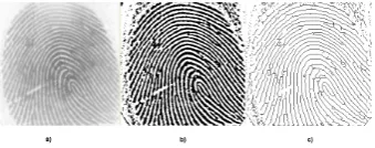
Fig. 9: Example of the result of the Stentiford thinning algorithm applied to a fingerprint image. a) fingerprint image; b) binarized image; c) thinned image.

of binarized fingerprints, in a grayscale, where the information of interest such as the pixels in black are processed in a window of 3 rows by 3 columns. Soon after the black pixel receives the white color, that is, it is deleted, when all the conditions below are true.

3.3.1 Stentiford thinning algorithm. In 1983, Stentiford intro-duced a new approach for skeletonization algorithms using a mask concept. Four masks are used to scroll the image in an orderly man-ner in the form: M1, M2, M3, M4. The four different masks used in the algorithm Stentiford are shown in Figure

The white circle represents a white pixel with a value of 255 in Figure 8. The black circle represents a black pixel with a value of zero and the ”X” represents a pixel that is either black or white, that is it is indifferent. These masks cross the image in the following order:

—M1 - from left to right and top to bottom; —M2 - from bottom to top and from left to right; —M3 - from right to left and from bottom to top; —M4 - from top to bottom and from right to left.

The steps of the Stentiford algorithm are:

(1) Scroll the image until a pixel that fits the mask M1 is found; (2) If this pixel is not an end point, and if its number is connectivity

= 1, mark this point to be deleted afterwards.; (3) Repeat steps 1 and 2 for all pixels that fit in mask M1; (4) Repeat steps 1, 2 and 3 for each mask M2, M3 and M4 in this

order;

(5) If any item is marked to be deleted, it must be cleared by changing it to white;

(6) If any item was deleted in step 5;

(7) Repeat all steps from step 1 if not, the process ends.

The results of the thinning processing of the Stentiford algorithm are shown in Figure 9

3.3.2 Holt thinning algorithm. Most of the thinning algorithms work by successive applications of a set of rules in an image. In 1987, Holt suggested a new and faster algorithm that does not in-volve iterations, by writing the two iterations in logical expressions and using a 3x3 neighborhood.

Fig. 10: location of points around a central pixel.

Fig. 11: Example of the Holt thinning algorithm applied to a fingerprint image. a) original fingerprint; b) binarized image; c) thinned image.

The idea is to transform both sets of rules proposed by Zhang Suen into a single logical expression. The two iterations used in the Zhang algorithm are represented in equations 23 and 24.

v(C)∧(∼edge(C)∨(v(L)∧v(S)∧(v(N)∨v(O)))) (23)

v(C)∧(∼edge(C)∨(v(O)∧v(N)∧(v(S)∨v(L)))) (24) where v (C) represents the point value, so that the result will be true if the point is black and false if white; edge (C) checks if the point is on the edge of the image; The letters C, L, O, N, S represent the positions of pixels around the center point (C) as shown in Figure 10.

The algorithm executes the first iteration and then the second; both algorithms are based on Zhang Suen. The results of the thinning processing of the Holt algorithms are shown in Figure 11.

3.4 Minutiae extraction process

One of the most widely used techniques for the detection of minu-tiae is known as the Crossing Number (CN)[10].

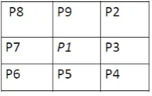
This technique determines the properties of a pixel simply by counting the number of existing black and white transitions in the neighborhood of the pixel (P) being processed. The Crossing Num-ber of a point P is given by Equation 25.

CN(p) = 0,5· X

i=1...8

val(p(i mod8))−val(p(i−1)) (25)

where p0, p1, ..., p7 are the pixels belonging to the sequence around the central pixel (P) with the central 8x8 neighborhood. val(p) is the value of each pixel. Therefore, to determine which at kind of minutia detail is present it is only necessary enough to analyze the neighborhood of each pixel through the CN(p) value.

Fig. 12: Example of detection of minutiae in a thinned binarized image. The square dots represent minutiae points (bifurcations).

4. COMPARATIVE ANALYSIS OF IMPLEMENTED ALGORITHMS

This chapter describes the results of comparative analysis of the techniques of thresholding, thinning and automatic recognition of minutiae points of bifurcation or termination without the prepro-cessing steps before binarization.

4.1 Evaluation criteria for the binarization process

The runtime of the algorithms and the quality of the images ob-tained in the binarization step are evaluated based on the theories of digital printing and the theory of algorithm binarization and thin-ning

Samples of digitized images in a bank of fingerprint images taken from students aged 20 to 30 years old are obtained to evaluate these criteria.

The samples are divided into two groups: group A (GA) and group B (GB), where each group consists of 80 samples of digital images of 10 fingers, eight images were made of each finger in different positions on the sensor.

The type of sensor to acquire the images was different for the two groups; however format (. * Bmp), resolution (500 dpi) and number of samples (80) were the same for the two groups as shown in Table 1. The following criteria were considered in the results:

—Image quality resulting from the binarization process (qualita-tive);

—Runtime;

—Size of the neighborhood used in the algorithms of adaptive lo-cation threshold;

—Number of minutiae points.

Table 1. : Features of the images in groups A and B.

A score ranging from one (1) to five (5) was used to measure the quality, where (1) is the worst, and (5) the best. Various characteris-tics were evaluated in the images, such as: the ridges, deltas, bifur-cations, intersections, spurs and terminations. A score is assigned to each image through a visual analysis by a group of 10 people, and the final result is the average scores given by the group.

The average runtime on 100 successive runs of each algorithm was used for the runtime performance of the algorithms.

In the Bernsen and Niblack algorithms, windows of 5x5 and 15x15 neighborhoods were used to calculate the threshold (T) for each pixel.

4.2 Results of the thresholding algorithm analysis

First, the two characteristics evaluated in groups A and B, of the fingerprints images, were the quality and the runtime of the algo-rithms. The conversion of the gray level image for a binarized im-age is of fundamental importance for the subsequent thresholding processes.

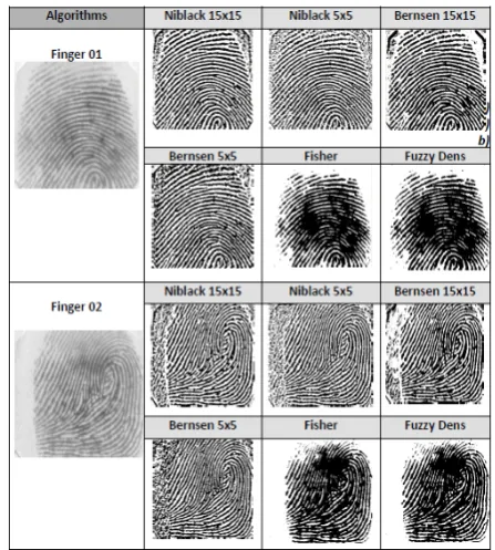
However the images binarized by the algorithms should show the highest level of detail with good definition of the ridges and valleys without any loss of information. For the group A images taken us-ing an optical sensor, the global thresholdus-ing algorithms had better qualitative results. For the group B images taken using a capacitive sensor, the local threshold algorithms are highlighted.

4.2.1 Quality of the image after the binarization process (qualita-tive). The algorithms that gave the best results in binarization qual-ity for the GA images were the Niblack and Bernsen algorithms, both with 15 15 neighborhood. Dens fuzzy algorithm produced the best results in the GB images. However, the Niblack algorithm with 5 5 neighborhood produced the worst picture quality featuring many irregularities.

The results of each binarization algorithm are illustrated in Table 2, showing the quality differences using two different fingers.

Fig. 13: Result of Stentiford thinning. a) fingerprint; b) binarization; c) thin-ning.

4.2.2 Runtime. The Fuzzy algorithm had the fastest threshold runtime, while the Niblack algorithm with a 15 15 neighborhood was the slowest, followed closely by Bernsen 5 5.

Table 3 illustrates the results of the averaged time (T) and quality (Q) for the binarization process of the images of groups A (GA) and B (GB).

Table 3. : Quality and Runtime results of the eight algorithms.

4.2.3 Neighborhood size used in local adaptive thresholding al-gorithms. The algorithms, Niblack and Bernsen, were subjected to two sizes of windows 5x5 and 15x15. As the window increases, the amount of pixels to be processed for the calculation of the local threshold increases, resulting in more time spent on image bina-rization.

4.3 Results of analysis of thinning algorithms

The two thinning algorithms evaluated were: Stentiford and Holt. The results obtained by the algorithm Stentiford were not satisfac-tory for this type of application of fingerprint images due to the presence of pixel discontinuities. On the other hand, this remains a faithful thinning of the lines with high curvature and points that are very close together. Figure 13 shows the results of the Stentiford thinning technique.

The second thinning algorithm, Holt, gave better results, and was faster and simpler to implement. The results of the Holt thinning technique are presented in Figure 14.

4.4 Results of minutiae extraction analysis

This step is one of the most important in a system of fingerprint recognition, because the details are the characteristics that define the uniqueness of each person and are directly related to the classi-fication and comparison of minutiae.

A major problem in comparing minutiae is image noise that may be generated by many factors such as dirt, excess moisture, low

Fig. 14: Result of Holt thinning. a) fingerprint; b) binarization; c) thinning.

Fig. 15: Result of bifurcation type minutiae extraction applied to an image with median filter pre-processing. a) original image; b) binarized image; c) sharpened image; d) extraction of minutiae.

quality. One of the problems this noise can cause in an AFIS (Au-tomatic Fingerprint Identification System) system is to recognize false minutiae points or to find non-existing points in a fingerprint. However, one way to solve this problem is by preprocessing which removes this noise.

The results of extracting bifurcation type minutiae applied to an image with median filter pre-processing are shown in Figure 15. Locations of the two forms of ridges in fingerprint images: bifurca-tion and terminabifurca-tion are tested using the CN algorithm. Both minu-tiae are found satisfactorily, and the only factor that hinders this is the noise in the original image.

5. CONCLUSION

This paper describes the main techniques of image processing used in a system for fingerprint recognition that seeks termination and bifurcation minutiae, in order to eliminate any possibility of false results.

The tests are based on the following criteria: image quality result-ing from binarization processes (qualitative); runtime; size of the neighborhood used in the algorithms of adaptive threshold loca-tion and a sufficient number of minutiae points. To obtain enough minutiae points, it is necessary to implement the thinning technique and process it after the binarized image with two algorithms: Sten-tiford and Holt. We recommend that the noise in the images should be completely removed so that the system can reliably extract the minutiae. However, it is fundamentally important to apply appro-priate preprocessing techniques to generate reliable results.

6. REFERENCES

[1] J. Bernsen. Dynamic thresholding of gray level images. In-ternational Conference on Pattern Recognition, pages 1251– 1255, 1986.

[2] C. Coetzee, C. Botha, and D. Weber. Pc based number plate recognition system. InIndustrial Electronics, 1998. Proceed-ings. ISIE ’98. IEEE International Symposium on, volume 2, pages 605–610 vol.2, Jul 1998.

[4] Edward Richard Henry. Classification and Uses of Finger Prints. HMSO, 2 edition, 1900.

[5] Lei Huang, Genxun Wan, and Changping Liu. An improved parallel thinning algorithm. InDocument Analysis and Recog-nition, 2003. Proceedings. Seventh International Conference on, pages 780–783, Aug 2003.

[6] A.K. Jain, Lin Hong, S. Pankanti, and R. Bolle. An identity-authentication system using fingerprints. In Proceedings of the IEEE, volume 85, pages 1365–1388, September 1997. [7] Anil Jain, Lin Hong, and Sharath Pankanti. Biometric

identi-fication.Communications of the ACM, 43(2):90–98, 2000. [8] Zhang Jinhai. Study and implementation of automatic

finger-print recognition technology. InUncertainty Reasoning and Knowledge Engineering (URKE), 2011 International Confer-ence on, volume 2, pages 40–43, Aug 2011.

[9] S. Philipp J.P. Coquerez, editor.Analyse d’images : filtrage et Segmentation. Masson, 1995.

[10] D. Maltoni, D. Maio, A. K. Jain, and S. Prabhakar.Handbook of Fingerprint Recognition. Springer Press, 2 edition, 2005. [11] W. Niblack.An Introduction to Digital Image Processing.

En-glewood Cliffs, N.J., 1986.

[12] S. Pankanti, R.M. Bolle, and A Jain. Biometrics: The fu-ture of identification [guest eeditors’ introduction].Computer, 33(2):46–49, Feb 2000.

[13] TI ON. Wsq gray-scale fingerprint image compression speci-fication, February 1993.

[14] Flavio Maggessi Viola. Estudo sobre formas de melhoria na identificao de caractersticas relevantes em imagens de im-presso digital. Master’s thesis, Universidade Federal Flumi-nense, August 2006.