http://dx.doi.org/10.4236/ijg.2015.610090
Correspondence Analysis on a
Space-Time Data Set for Multiple
Environmental Variables
Palma Monica
Universitá del Salento, Lecce, Italy Email: [email protected]
Received 3 August 2015; accepted 26 October 2015; published 29 October 2015
Copyright © 2015 by author and Scientific Research Publishing Inc.
This work is licensed under the Creative Commons Attribution International License (CC BY). http://creativecommons.org/licenses/by/4.0/
Abstract
Applications of the multivariate technique called correspondence analysis for environmental stu-dies are relatively new and are limited to spatial multivariate data set. In this paper, a procedure of applying correspondence analysis to a large space-time data set for multiple environmental va-riables is shown. In particular, nitrogen dioxide and carbon monoxide hourly concentrations measured during January 1999 at several monitored stations in a district of Northern Italy are analyzed. The procedure consists in transforming the continuous variables into categorical ones by the means of appropriate indicator variables, generating special contingency tables and apply-ing correspondence analysis. The use of this classical multivariate technique allows the identifica-tion of important relaidentifica-tionships among polluidentifica-tion levels and monitoring staidentifica-tions and/or relaidentifica-tion- relation-ships among pollution levels and observation times.
Keywords
Space-Time Data, Indicator Transform, Correspondence Analysis
1. Introduction
Usually environmental monitoring networks collect a huge amount of data such as pollutant concentrations, atmospheric variates, weather conditions, and so on, which are of particular interest for public policies oriented to environmental and human health protection.
Such data sets may have the following features:
• they are multivariate, as several variables are simultaneously measured;
and for a certain period of time.
Classical multivariate techniques represent useful tools for analyzing multiple va-riables. Their main goal is to obtain a summary description of the data: Principal Component Analysis (PCA) finds a smaller number of variates representing all those collected, without loss of essential information; Correspondence Analysis (CA) studies the association between two or more categorical variables by representing the categories of the variables as points in a low-dimensional space; Canonical Correlation Analysis (CCA) describes the relationships between two groups of several variables. Classical multivariate techniques can be also applied to space-time data sets in order to summarize the spatial and temporal profiles which characterize the information, finding relationships among the data. In De Iaco et al. [1], the use of PCA allowed summarizing a very large data set of space-time observations for three contaminants. The authors identified a single measure of total air pollution which synthesized the original data without loss of information. Moreover, lately a space-time data set for air pollution and atmospheric variables has been analyzed through CCA in De Iaco [2]. The author emphasized the features of that multiva-riate technique which allowed describing very important relationships between three contaminants (nitrix oxide, nitrogen dioxide and ozone) and atmospheric indicators (humidity, temperature and wind speed).
Hence, when multiple variables are measured at several locations of the area under study and for a period of time, in other words, when a space-time multivariate data set is available, and the aim is studying the simul- taneous behaviour of the va-riables in order to understand the relationships among the space-time observations, a multivariate technique is the most useful tool. CA is one of the multivariate techniques with a wide range of applications in several fields such as social and political sciences, marketing research, economy, ecology and biology. This technique is usually applied as an exploratory method, with the aim to describe the structure of the data under study with minimal constraints on the form of the same structure [3].
In this paper, it will be shown that even CA can be applied to a space-time multivariate data set, finding very important results which other techniques may not highlight. In particular, in this paper CA will be applied to an air pollution data set involving two contaminants measured at monitoring stations in northern Italy during January 1999. The analysis will identify relationships in space among pollution levels and monitoring stations and relationships in time among pollution levels and observation times.
After a presentation of CA (Section 2) and a review of its theory (Section 2.1), the description of compu- tational aspects follows (Section 2.2). Then, the data set (Section 3) and the most important results from the applied CA and their interpretation are given (Section 4).
2. Correspondence Analysis
CA is an algebraic technique analogous to PCA, but, while PCA is used for tables of continuous measurements, CA is more appropriate for categorical variates. Hence, CA is suitable for analyzing qualitative information represented by a contingency table. Lebart et al. [4] suggest that CA is useful for the analysis of large data matrices, particularly when there is little auxiliary information concerning the data. The original development of the method was driven by the need to analyze occurrence frequencies in a contingency table [5]. This technique can be viewed as finding the best simultaneous representation of two data sets that comprise the rows and columns of a data matrix with non-negative entries [4].
For a long time CA has been applied by European statistical community for psycho-metric and economic studies. This technique has been very popular in France, mainly owing to the efforts of Jean-Paul Benzécri [5]; it came to occupy such a strong position in the analysis methodology that it almost became synonymous with data analysis. In the 80’s this technique started to be used in English-speaking countries since some books and papers presented the method in relatively simple form [4] [6] and now several American statistical package, such as SAS [7] and SPSS [8], include procedures to perform correspondence analysis. In the geostatistical context, applications of CA are relatively new. Avila et al. in [9] and [10] analyzed a data set consisting of the concen- trations of chemical elements measured in a lake; Dutot et al. [11] applied this method to an aerosol collected in a simple atmospheric environment; Jiménez-Espinosa et al. [12] used CA on 602 soil samples taken in a region of NW Spain to identify geochemical patterns and anomalies.
within the observed period which need of closer controls because of frequent exceeding fixed pollution levels, is definitely a very important issue. CA allows achieving this goal simultaneously for several contaminants. Therefore, it is useful to develop a procedure of applying CA to space-time multivariate data sets.
2.1. The Method
The theory of CA is discussed in several books, [4]-[6], so only the main features of the method are reviewed here.
From an initial data matrix X(l p× ) with non-negative entries xhi,h=1,, ;l i=1,,p, CA determines the
best simultaneous geometrical representation of rows and columns in a low-dimensional space (usually in a two- dimensional space).
Let F(l p× ) be the relative frequency matrix, whose entries are:
1 1
.
p l hi hi hi
h i
f x x
= =
=
∑∑
(1)Two different matrices are used to re-scale F, these are:
[ ]
diag l = fh⋅D (2)
and
[ ]
diag , p = f⋅iD (3)
where:
1
, 1, ,
p h hi
i
f ⋅ f h l
=
=
∑
∀ = (4)and
1
, 1, , .
l i hi
h
f⋅ f i p
=
=
∑
∀ = (5)CA consists in finding a vector u, in a p-dimensional space, which maximizes
T
T 1 1 1 1
,
l p l l p
− − − −
u D FD D D FD u (6)
subject to the constraint:
T 1
1. p
− =
u D u (7)
It is known that this is equivalent to finding the vector v, in an l-dimensional space, which maximizes
T
T 1 T 1 1 T 1
,
p l p p l
− − − −
v D F D D D F D v (8)
subject to the constraint:
T 1
1. l
− =
v D v (9)
The eigenvectors u and v are related by:
1 T 1
1 1 and p l λ λ − − = =
v FD u u F D v (10)
where λ is the same eigenvalue for either maximization problems in (6) and (8).
This duality formula permits displaying the row and column projections in the same graph (called biplots) and this CA feature has been considered as its advantage with respect to others multivariate techniques.
Sequentially, the method searches for new solutions orthogonal to the previous ones; in particular, orthogo- nality is considered with respect to the inner product defined by the weighting matrices (2) and (3). There will be
(
min ,( )
l p −1)
non-trivial solutions.1
p −
Φ =D u (11)
and
1
l −
Ψ =D v (12)
define the plane where rows and columns of the data matrix are projected.
Results from CA consist of graphical representations of the projections of rows and columns of the data matrix onto factorial planes, in order to find and understand underlying relationships [4]. There are also con- venient diagnostics that help in the interpretation of the results; in particular:
• the percentage of explained variation, which is a measure of fit when a particular factor is retained, so that the cumulative percentage of explained variation
( )1
min , 1
1 , K k k l p k k λ λ = − =
∑
∑
(13)represents a global measure of fit when K factors,
(
K<min ,( )
l p −1)
are retained, each λk giving the contribution of a particular factor. Note that the terminology is similar to that one used in PCA, but in CA the term variation does not refer to variance in the statistical sense; it is an increasing function of K and it is used to choose the number of factors to be kept;• the absolute contributions of the h-th row
( )
AC kh and the i-th column( )
AC ik to the k-th factor,( )
(
)
1, , min , 1
k= l p − , explain the composition of the retained factor. They are respectively:
(
)
21, , ,
k
h hk h
AC = f ⋅ψ h= l (14)
and
( )
21, , ;
k i ik i
AC = f⋅φ i= p (15)
• the relative contributions of a retained factor with the h-th row
( )
k hRC or the i-th column
( )
k iRC provide a measure of the row or column variation explained by the factor. They are respectively:
( )
min ,( )122 1
1, , ,
k k hk h l p
k hk k
RC λ ψ h l
λ ψ − = = =
∑
(16) and( )
min ,( )122 1
1, , .
k k ik i l p
k ik k
RC λ φ i p
λ φ − = = =
∑
(17)Note that the ACs serve primarily as guides to the interpretation of the dimension defined by the retained factors; whereas the RCs indicate how well a point is described by the retained factors. Usually, a large AC implies a large RC, but not conversely [6].
2.2. Computational Aspects
The application of CA to a space-time data set for multiple environmental variables is based on special con- tingency matrices generated as follows.
Let zr
(
sα ω,t)
,r=1,, ;R sα =( )
x y, α∈ ⊂ ℜD 2;tω∈ ⊂ ℜT , be the space-time data for R variablesmeasured at α-th location, α =1,,Nr and ω-th observation time, ω=1,,W . For semplicity, consider , 1, , ,
r
Let r, 1, , ; 1, , , j
c j= J r= R be J non-overlapping classes of values defined for each of the R variables under study.
Through the indicator transform, the belonging of z s tr
(
α ω,)
to a certain class of values is described:(
)
1 if(
,)
,, , 0 otherwise. r r j r r j
z t c
i α tω c = α ω ∈
s
s (18)
From the four dimensional matrix (variable, station, time, class of values) obtained after the indicator trans- formation (18), the following two dimensional matrices are generated.
• Matrix ( ) r, j R N× ×J = nα
A , where
(
)
, 1 , , , W r rj r j
nα i α tω c
ω=
=
∑
s (19)1, ,N j; 1, , ;J r 1, , .R
α = = =
In A, the
(
R N×)
rows represent all survey stations for each variable and the columns represent the J classes of values, so that the entries (19) indicate the number of times, values belonging to the j-th class, are recorded at the α-th station.• Matrix ( ) ,
r j R W× ×J = mω
B , where
(
)
, 1 , , , N r rj r j
mω i α tω c
α=
=
∑
s (20)1, ,W j; 1, , ;J r 1, , .R
ω= = =
In B, the
(
R W×)
rows represent the observation times for each variable and the columns represent the J classes of values, so that the entries (20) indicate, for each variable, how many stations in the ω-th observation time have values belonging to the j-th class.The indicator transform allows the user to categorize continuous variables, synthesizing a large multivariate space-time data set. The above two dimensional matrices relate different classes of values (in the case study pollution levels) to locations (matrix A) or to observation times (matrix B), jointly for the variables (pollutants) under study. Thus, CA applied to each matrix, A and B, will allow describing relationships
• in space, among pollution levels and monitored stations, • in time, among pollution levels and observation times, simultaneously for the variables under study.
CA results will also identify clusters of survey stations and intervals of time which need of closer controls when the contaminants frequently exceed fixed thresholds.
3. The Data Set
The data set consists of concentration values of two pollutants over a particular period of time and at stations of the monitoring network in Milan district, Lombardy (this is one of the northern Italy regions which suffers a serious air pollution pro-blem). The air quality monitoring network covers a wide area with about 190 stations where the main atmospheric contaminants, such as sulphur dioxide (SO2), ozone (O3), nitric oxide (NO),
nitrogen dioxide (NO2), carbon monoxide (CO), and meteorological variates, such as humidity, wind velocity,
temperature, solar radiation, are continuously measured.
In the Milan district, air pollution is mainly caused by traffic and industrial activities. Two pollutants, which are primarily generated by the human activities, considered among the most dangerous ones for the atmosphere and human health and have been analyzed in this paper: NO2 and CO. Nitrogen dioxide is a secondary pollutant
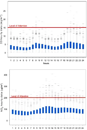
the hourly averages for each pollutant, measured during January 1999 (Figure 1), highlights exceeding the so called level of attention for several times during the month.
The national laws, particularly the Premier’s Decree of the 12th of November, 1992, according to the European settlements, lay down, for each pollutant, a specific threshold called level of attention. When the pollution concentrations exceed this level for a long time and at several monitoring stations, air quality is poor and the situation is considered dangerous for the public health.
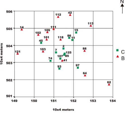
The analysis is limited to stations in the Milan district where data for both contaminants are available at all the desidered time points. In Figure 2, the 27 selected survey stations are shown. They have been classified, according to the Premier’s Decree of the 20th of May, 1991, in two types:
• stations C, which are located in areas with heavy traffic and poor ventilation; in these areas the CO plume is more evident;
[image:6.595.168.464.249.689.2]• stations B, which are located in areas with high density population, therefore these areas are subject to both NO2 and CO pollution.
Figure 2. Posting map of the selected survey stations in Milan district.
In order to split each spatial-temporal distribution into non-overlapping classes of values, the following thresholds:
a) 1.6 2.3 3 3.9 5.4 mg/m3 b) 52 64 75 90 115 µg/m3
corresponding to the 0.17, 0.33, 0.50, 0.67, 0.83 quantiles of the distributions of CO a) and NO2 b) hourly
averages, are considered. Hence, six classes of CO and NO2 concentrations are defined as follows:
(
)
1 minimum , ; 0.17 quantile value
r
r
c = z sα tω
(
1)
quantile value; quantile value , 2, , 5;
6 6
r q
q q
c = − q=
(
)
6 0.83 quantile value; maximum , ,
r
r
c = z sα tω
1, 2; 1, , 27; 1, , 744.
r= α= ω=
Then, through the indicator transform, two dimensional matrices are generated as described in (2.2); so that: • A is a
(
2 27×)
× =6 54 6× matrix, whose entries are:(
)
744 ,
1
, ;
r r
j r j
nα i α tω c
ω=
=
∑
s (21)1, , 27;j 1, , 6;r 1, 2
α = = = ;
• B is a
(
2 24×)
× =6 48 6× matrix, whose entries are ,r j
mω , as defined in (20), cumulated every 24 hours, that is:
(
)
30 27 ,
0 1
ˆr j r , 24 ; rj
mω i α tω c
δ α
δ
= =
=
∑∑
s + (22)1, , 24;j 1, , 6;r 1, 2.
ω= = =
CA is applied to these matrices.
4. Results
techniques, giving graphical results and diagnostics, in a very simple and fast manner.
Even if it is a commercial software, it is a very powerful software for data mining, indeed it can perform many statistical data analysis, as Factorial Analysis, Classification, Segmentation, as well as Textual analysis. Moreover, SPAD has a good graphical tools and is easy to use (user-friendly) [17].
CA is applied to matrix A and matrix B, since information from both analysis are useful for the aim of the paper, as it will be shown.
The results from CA are displayed in a series of tables and graphs. In particular, Table 1andTable 2show the eigenvalues and the percentages of variation explained by the five non-trivial factors from CA applied to the matrix A and B, respectively.
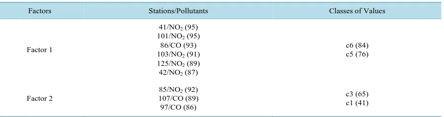
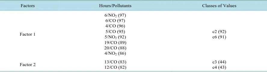
On the other hand, Table 3 and Table 4 list, for the first two factors from CA applied to the matrix A, stations/pollutants with the highest absolute (Table 3) and relative (Table 4) contributions. Similarly Table 5 and Table 6, which refer to the diagnostics from CA applied to the matrix B.
Figure 3 and Figure 4 show the projections of rows and columns of each matrix on the respective first factorial plane. Note that in Figure 3, which refers to matrix A, columns (points labeled 1,c , 6c ) and rows (points labeled with the station code and a symbol related to the pollutants) are displayed together on the same plane. Similarly in Figure 4, where columns (points c1,, 6c ) and rows (observation hours, 1,, 24, labeled with different symbols for the pollutants under study) of the matrix B are projected together on the same plane.
Figure 3. Plot of the first two factors from CA applied to the matrix A.
Table 1. Eigenvalues and percentages of variation explained by the factors from CA applied to the matrix A.
Eigenvalues Variation Explained (%)
Factor 1 0.0975 59.90
Factor 2 0.0408 25.05
Factor 3 0.0161 9.89
Factor 4 0.0048 2.94
[image:9.595.87.535.231.340.2]Factor 5 0.0036 2.22
Table 2. Eigenvalues and percentages of variation explained by the factors from CA applied to the matrix B.
Eigenvalues Variation Explained (%)
Factor 1 0.0951 85.26
Factor 2 0.0115 10.29
Factor 3 0.0030 2.69
Factor 4 0.0013 1.21
[image:9.595.93.538.373.509.2]Factor 5 0.0006 0.56
Table 3. Highest absolute contributions to the first two factors from CA applied to the matrix A (percentages in paren-theses).
Factors Stations/Pollutants Classes of Values
Factor 1
86/CO (11) 15/CO (8) 41/NO2 (8)
93/CO (5) 45/CO (4) 125/NO2 (4)
c6 (39) c1 (29)
Factor 2
97/NO2 (27)
62/CO (9) 97/CO (7) 111/CO (6)
[image:9.595.92.541.542.661.2]c1 (50) c3 (21)
Table 4. Highest relative contributions to the first two factors from CA applied to the matrix A (percentages in
paren-theses).
Factors Stations/Pollutants Classes of Values
Factor 1
41/NO2 (95)
101/NO2 (95)
86/CO (93) 103/NO2 (91)
125/NO2 (89)
42/NO2 (87)
c6 (84) c5 (76)
Factor 2
85/NO2 (92)
107/CO (89) 97/CO (86)
c3 (65) c1 (41)
The position of the points and the absolute and relative contributions suggest the following comments.
CA applied to the matrix A.
As previously described, matrix A relates six non-overlapping classes of values to CO and NO2 survey
Table 5. Highest absolute contributions to the first two factors from CA applied to the matrix B (percentages in parentheses).
Factors Hours/Pollutants Classes of Values
Factor 1
6/NO2 (7)
5/NO2 (6)
6/CO (6) 5/CO (6) 4/NO2 (5)
19/CO (5) 20/CO (5) 4/CO (4)
c6 (42) c1 (32)
Factor 2
12/CO (9) 13/CO (7) 13/NO2 (7)
12/NO2 (4)
c6 (34) c1 (25)
Table 6. Highest relative contributions to the first two factors from CA applied to the matrix B (percentages in parentheses).
Factors Hours/Pollutants Classes of Values
Factor 1
6/NO2 (97)
6/CO (97) 4/CO (96) 5/CO (95) 5/NO2 (92)
19/CO (89) 20/CO (88) 4/NO2 (86)
c2 (92) c6 (91)
Factor 2 13/CO (83)
12/CO (82)
c3 (44) c4 (43)
different pollution levels and monitored locations. The first two factors are retained since they explain together about 85% of the total variation (Table 3).
The last class of values (c6) and the first one (c1) have the highest absolute contributions to the first factor, respectively, 39% and 29% (Table 2); whereas the first class (c1) and the third one (c3) have the highest absolute contribution to the second factor (respectively, 50% and 21%). Hence, the first factor better explains the variation of high pollution levels, i.e. levels which are greater than the last quantile values (5.4 mg/m3 for CO and 115 µg/m3 for NO2), while the second factor better explains the variation of low pollution levels, i.e.
levels which are smaller than 1,6 mg/m3 for CO and 52 µg/m3 for NO2. Table 2list also the stations/pollutants
which have the highest absolute contributions to the retained factors. The first factor better represents stations located at the central area of the Milan district (86, 125, 41, 93, 15), while the second factor better represents stations located at the peripheral areas (62, 97, 111).
The cumulative relative contributions to the first two factors (Table 4shows those stations/pollutants and classes with the highest relative contributions) are always greater than 80%, highlighting the good quality of representation of rows and columns in the space determining by the first two factors.
The projection of the classes to the first factorial plane (Figure 3) shows a horseshoe effect [6] which corresponds to a non-linear relationships between the two axes, even if they are linearly orthogonal.
In Figure 3, classes and stations/pollutants are displayed together so that and it is possible to identify two clusters of stations/pollutants:
1) points 111, 11, 45, 81, referred to CO, and point 41, referred to NO2, with positive first and second
co-ordinate;
2) points 86, 15, 93, 113, 101, referred to CO, and points 102, 15, referred to NO2, with negative first
co-ordinate.
The position of the second cluster on the factorial plane, being the points closer to point c6 with respect to the other points, highlights that most of the highest pollutant concentrations was read during January 1999 at those locations.
CA applied to the matrix B.
[image:10.595.94.538.268.389.2]monitoring stations, at a fixed hour, have recorded pollution levels belonging to a given class of values. Hence, by analyzing this matrix, underling relationships among observation times (hours) and different pollution levels can be identified.
Table 2 shows the eigenvalues and the percentages of variation explained by each of the 5 non-trivial factors. In this case, the first factor explains a greater part of the total variation (85.26%) than in the previous analysis. The greater the percentage of explained variation, the greater the association between rows and columns of the data matrix, then the high percentage of variation explained by this factor is due to a strong association between observation times and classes of pollution levels. Once more, the first two factors are retained since they explain together more than 95% of the total variation.
Figure 4shows the projections of rows (hours/pollutants) and columns (classes of values) to the first factorial plane. Now, a horseshoe effect is evident not only in the projections of the classes, but also in the projections of the hours/pollutants on the factorial plane: this means that distant pairs of hours can be considered as equidistant, while neighbouring hours are progressively dissimilar.
Table 5 and Table 6list the classes of values and the hours/pollutants with the highest absolute (Table 5) and relative (Table 6) contributions. Hours 4, 5, 6 referred to both contaminants have the highest absolute contribu- tions to the first factor and, by looking to the factorial plane (Figure 4), the position of these observation times closer to point c1 with respect to the other points highlights that most of CO and NO2 low readings was
measured from the 4-th to the 6-th hour. Instead, most of the high pollution concentrations was observed during the evening, particularly during the 19-th to the 22-nd hour, for CO and from the 12-th to 14-th hour, for NO2.
5. Conclusion
In this work, an application of CA to an air pollution space-time data set for CO and NO2 hourly concentrations,
recorded at some monitoring stations in Milan district, is given. The transformation of the original continuous variables into new categorical ones has been formally presented in this paper by the means of the indicator approach. By counting the indicator data over both spatial locations and observation times, two contingency matrices are generated. Each of them accounts information of both pollutants examined in this paper. CA is applied to these matrices providing a summary description of spatial and temporal profiles, simultaneously for the contaminants under study. The data analysis allows identifying relationships in space among CO and NO2
pollution levels and monitored stations and relationships in time among CO and NO2 pollution levels and
observation times. The aim of each air quality control system is to obtain information about the atmospherical conditions and evaluate the opportunity of major restrictions and closer controls. The application of CA carried out in this paper makes it possible, since its graphical results and diagnostics help in identifying stations inside the area under study and intervals of time during the day for which the contaminants of interest need closer controls because of joint exceeding of fixed pollution levels.
Acknowledgements
The author would like to thank Prof. Donato Posa of University of Salento, Apulian region (Italy), whose suggestions have been helpful and improved this paper.
References
[1] De Iaco, S., Myers, D.E. and Posa, D. (2000) Total Air Pollution and Space-Time Modeling. In: Monestiez P., Allard D. and Froidevaux R., Eds., GeoEnv III, Geostatistics for Environmental Applications, Kluwer Academic Publishers, Norwell, 45-56.
[2] De Iaco, S. (2011) A New Space-Time Multivariate Approach for Environmental Data Analysis. Journal of Applied Statistics, 38, 2471-2483. http://dx.doi.org/10.1080/02664763.2011.559206
[3] Blasius, J., Greenacre, M., Groenen, P.J.F. and van de Velden, M. (2009) Special Issue on Correspondence Analysis and Related Methods. Computational Statistics and Data Analysis, 53, 3103-3106.
http://dx.doi.org/10.1016/j.csda.2008.11.010
[4] Lebart, L., Morineau, A. and Warwick, K.M. (1984) Multivariate Descriptive Statistical Analysis. John Wiley & Sons, New York.
[6] Greenacre, M.J. (1989) Theory and Applications of Correspondence Analysis. Academic Press, London. [7] SAS/Stat (1990) SAS Institute Inc., Cary.
[8] (1999) SPSS 8.0, SPSS Inc., Chicago.
[9] Avila, F. and Myers, D.E. (1991) Correspondence Analysis Applied to Environmental Data Sets: A Study of Chautau-qua Lake sediments. Chemometrics and Intelligent Laboratory Systems, 11, 229-249.
http://dx.doi.org/10.1016/0169-7439(91)85002-7
[10] Avila, F., Myers, D.E. and Palmer, C. (1991) Correspondence Analysis and Adsorbate Selection for Chemical Sensor Arrays. Journal of Chemometrics, 5, 455-465. http://dx.doi.org/10.1002/cem.1180050505
[11] Dutot, A.L., Bergametti, G. and Buat-Menard, P. (1988) Application of Correspondence Analysis to Apportion Sources of Ambient Particles. Athmospheric Environment, 22, 1737-1743. http://dx.doi.org/10.1016/0004-6981(88)90403-9
[12] Jiménez-Espinosa, R., Sousa, A.J. and Chica-Olmo, M. (1992) Application of Correspondence Analysis and Factorial Kriging Analysis: A Case Study on Geochemical Exploration in Geostatistics. 2, Soares, A. Ed., Troia, 853-864. [13] Greenacre, M.J. and Primicerio, R. (2013) Multivariate Analysis for Ecological Data. Fundación BBVA, Bilbao. [14] De Iaco, S., Palma, M. and Posa, D. (2013) Prediction of Particle Pollution through Spatio-Temporal Multivariate
Geostatistical Analysis: Spatial Special Issue. AStA Advanced Statistical Analysis, 97, 133-150.
http://dx.doi.org/10.1007/s10182-012-0199-0
[15] De Iaco, S., Maggio, S., Palma, M. and Posa, D. (2012) Advances in Spatio-Temporal Modeling and Prediction for Environmental Risk Assessment. In: Haryanto, B., Ed., Air Pollution—A Comprehensive Perspective, InTech, Croazia, 365-390. http://dx.doi.org/10.5772/51227
[16] (1999) SPAD 4.0, Cisia, Montreuil Cedex, France.