http://dx.doi.org/10.4236/ojfd.2015.53026
How to cite this paper: Mondal, R.N., Helal, M.N.A., Shaha, P.R. and Poddar, N.K. (2015) Time-Dependent Flow with Con-vective Heat Transfer through a Curved Square Duct with Large Pressure Gradient. Open Journal of Fluid Dynamics, 5, 238-255. http://dx.doi.org/10.4236/ojfd.2015.53026
Time-Dependent Flow with Convective
Heat Transfer through a Curved Square
Duct with Large Pressure Gradient
Rabindra Nath Mondal
1*, Md. Nurul Amin Helal
2, Poly Rani Shaha
1, Nayan Kumar Poddar
1 1Department of Mathematics, Jagannath University, Dhaka, Bangladesh2Additional Director (Education), Training Directorate, BGB Head Quarter, Pilkhana, Dhaka, Bangladesh Email: *[email protected]
Received 10 June 2015; accepted 22 September 2015; published 25 September 2015 Copyright © 2015 by authors and Scientific Research Publishing Inc.
This work is licensed under the Creative Commons Attribution International License (CC BY). http://creativecommons.org/licenses/by/4.0/
Abstract
A numerical study is presented for the fully developed two-dimensional laminar flow of viscous incompressible fluid through a curved square duct for the constant curvature δ = 0.1. In this paper, a spectral-based computational algorithm is employed as the principal tool for the simulations, while a Chebyshev polynomial and collocation method as secondary tools. Numerical calculations are carried out over a wide range of the pressure gradient parameter, the Dean number, 100 ≤ Dn ≤ 3000 for the Grashof number, Gr, ranging from 100 to 2000. The outer wall of the duct is treated heated while the inner wall cooled, the top and bottom walls being adiabatic. The main concern of the present study is to find out the unsteady flow behavior i.e. whether the unsteady flow is steady-state, periodic, multi-periodic or chaotic, if Dn or Gr is increased. It is found that the un- steady flow is periodic for Dn = 1000 at Gr = 100 and 500 and at Dn = 2000, Gr = 2000 but steady-state otherwise. It is also found that for large values of Dn, for example Dn = 3000, the unsteady flow undergoes in the scenario “periodic→chaotic→periodic”, if Gr is increased. Typical
contours of secondary flow patterns and temperature profiles are also obtained, and it is found that the unsteady flow consists of single-, two-, three- and four-vortex solutions. The present study also shows that there is a strong interaction between the heating-induced buoyancy force and the centrifugal force in a curved square passage that stimulates fluid mixing and consequently en- hance heat transfer in the fluid.
Keywords
Curved Square Duct, Secondary Flow, Time-Evolution, Periodic Solution, Chaos
1. Introduction
Fluid flow and heat transfer in curved ducts have been studied for a long time because of their fundamental importance in engineering and industrial applications. Today, the flows in curved non-circular ducts are of increasing importance in micro-fluidics, where lithographic methods typically produce channels of square or rectangular cross-section. These channels are extensively used in many engineering applications, such as in turbo-machinery, refrigeration, air conditioning systems, heat exchangers, rocket engine, internal combustion engines and blade-to-blade passages in modern gas turbines. In a curved duct, centrifugal forces are developed in the flow due to channel curvature causing a counter rotating vortex motion applied on the axial flow through the channel. This creates characteristics spiraling fluid flow in the curved passage known as secondary flow. At a certain critical flow condition and beyond, additional pairs of counter rotating vortices appear on the outer concave wall of curved fluid passages which are known as Dean vortices, in recognition of the pioneering work in this field by Dean [1]. After that, many theoretical and experimental investigations have been done; for instance, the articles by Berger et al. [2], Nandakumar and Masliyah [3], and Ito [4] may be referenced.
One of the interesting phenomena of the flow through a curved duct is the bifurcation of the flow because generally there exist many steady solutions due to channel curvature. Studies of the flow through a curved duct have been made, experimentally or numerically, for various shapes of the cross section by many authors. However, an extensive treatment of the bifurcation structure of the flow through a curved duct of rectangular cross section was presented by Winters [5], Daskopoulos and Lenhoff [6] and Mondal [7].
Unsteady flows by time evolution calculation of curved duct flows was first initiated by Yanase and Nishiyama [8] for a rectangular cross section. In that study they investigated unsteady solutions for the case where dual solutions exist. The time-dependent behavior of the flow in a curved rectangular duct of large aspect ratio was investigated, in detail, by Yanase et al. [9] numerically. They performed time-evolution calculations of the unsteady solutions with and without symmetry condition and found that periodic oscillations appear with symmetry condition while aperiodic time variation without symmetry condition. Wang and Yang [10] [11]
performed numerical as well as experimental investigation on fully developed periodic oscillation in a curved square duct. Flow visualization in the range of Dean numbers from 50 to 500 was carried out in their experiment. Recently, Yanase et al. [12] performed numerical investigation of isothermal and non-isothermal flows through a curved rectangular duct and addressed the time-dependent behavior of the unsteady solutions. In the succeeding paper, Yanase et al. [13] extended their work for moderate Grashof numbers and studied the effects of secon-dary flows on convective heat transfer. Recently, Mondal et al. [14] [15] performed numerical prediction of the unsteady solutions by time-evolution calculations for the flow through a curved square duct and discussed the transitional behavior of the unsteady solutions.
2. Mathematical Formulations
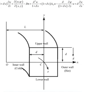
Consider an incompressible viscous fluid streaming through a curved duct with square cross section whose width or height is 2d. The coordinate system is shown in Figure 1. It is assumed that the temperature of the out-er wall is T0+ ∆T and that of the inner wall is T0− ∆T, where ∆ >T 0. The x, y, and z axes are taken to be in the horizontal, vertical, and axial directions, respectively. It is assumed that the flow is uniform in the axial di-rection, and that it is driven by a constant pressure gradient G along the center-line of the duct, i.e. the main flow in the axial direction as shown in Figure 1. The variables are non-dimensionalized by using the representative length d and the representative velocity U0=v d.
We introduce the non-dimensional variables defined as
0 0 0
2
, , , , ,
u v x y z
u v w w x y z
U U U d d d
δ ′ ′ ′ ′ ′ ′ = = = = = = 0 2 0
, U , , ,
T d P P
T t t P G
T d δ L ρU z
′ ′ ′ ∂ ′
= = = = = −
′
∆ ∂ ,
where, u, v and w are the non-dimensional velocity components in the x, y and z directions, respectively; t is the non-dimensional time, P the non-dimensional pressure, δ the non-dimensional curvature, and temperature is non-dimensionalized by ∆T. Henceforth, all the variables are nondimensionalized if not specified. The stream function ψ is introduced in the x- and y-directions as
1 1
, .
1 1
u v
x y x x
ψ ψ
δ δ
∂ ∂
= = −
+ ∂ + ∂ (1)
Then the basic equations for w,ψ and T are derived from the Navier-Stokes equations and the energy equation under the Boussinesq approximation as,
(
)
(
(
)
)
2(
)
2(
)
,
1 1 ,
, 1 1
w
w w w
x Dn x w w
t x y x x y x
ψ δ δ ψ
δ δ δ
δ δ
∂
∂ ∂ ∂
+ + − + = + ∆ − +
[image:3.595.204.426.205.266.2] [image:3.595.165.524.386.710.2]∂ ∂ + + ∂ ∂ (2)
(
)
(
( )
)
(
)
(
)
(
)
2 2
2 2 2 2
2 2 2
2 2 2 2 2 , 1 3 2
1 1 , 1 1
3 3 1 1 2 1 , 1
x x t x x y x y x x x
x x y x x x x
w T
w Gr x
x x y x
ψ ψ
δ ψ δ ψ ψ δ ψ ψ
δ δ δ δ
ψ ψ δ δ ψ δ ψ
δ δ
δ ψ ψ δ
δ ∂ ∆ ∂ ∂ ∂ ∂ ∂ ∆ − = − + ∆ − + + ∂ ∂ + ∂ ∂ + ∂ ∂ + ∂ ∂ ∂ ∂ − + × − ∂ ∂ ∂ + ∂ + ∂ ∂ ∂ ∂ − ∆ + + ∆ − + + ∂ ∂ ∂ (3)
(
)
(
(
)
)
2,
1 1
1 , Pr 1
T
T T
T
t x x y x x
ψ δ
δ δ
∂
∂ + = ∆ + ∂
∂ + ∂ + ∂ (4) where,
(
)
(
)
2 2 2 2 2
,
, .
,
f g f g f g
x y x y y x
x y
∂
∂ ∂ ∂ ∂ ∂ ∂
∆ ≡ + ≡ −
∂ ∂ ∂ ∂ ∂
∂ ∂ (5)
The Dean number Dn, the Grashof number Gr, and the Prandtl number Pr, which appear in Equations (2) to (4) are defined as
3 3
2
2
, , Pr
Gd d g Td
Dn Gr
L
β ν
µυ ν κ
∆
= = = (6) The rigid boundary conditions for w and ψ are used as
(
1,)
(
, 1)
(
1,)
(
, 1)
(
1,)
(
, 1)
0w y w x y x y x
x y
ψ ψ
ψ ψ ∂ ∂
± = ± = ± = ± = ± = ± =
∂ ∂ (7)
and the temperature T is assumed to be constant on the walls as
( )
1, 1,(
1,)
1,(
, 1)
T y = T − y = − T x ± =x. (8)
In the present study, Dn and Gr vary while Pr and δ are fixed as Pr = 7.0 (water) and curvature δ =0.1.
3. Numerical Calculations
3.1. Method of Numerical Calculation
In order to solve the Equations (2) to (4) numerically the spectral method is used. This is the method which is thought to be the best numerical method to solve the Navier-Stokes equations as well as the energy equation (Gottlieb and Orazag, [21]). By this method the variables are expanded in a series of functions consisting of the Chebyshev polynomials. That is, the expansion functions
( )
(
)
( )
( )
(
)
2( )
2 2
1 , 1
n x x Cn x n x x Cn x
φ = − ψ = − (9)
where Cn
( )
x =cos(
ncos−1( )
x)
is the nth order Chebyshev polynomial. w x y t(
, ,)
,ψ
(
x y t, ,)
and T x y t(
, ,)
are expanded in terms ofφ
n( )
x andψ
n( )
x as(
)
( ) ( ) ( )
(
)
( ) ( ) ( )
(
)
( ) ( ) ( )
0 0 0 0 0 0 , , , , , , , , , M Nmn m n
m n
M N
mn m n
m n
M N
mn m n
m n
w x y t w t x y
x y t t x y
T x y t T t x y x
φ φ
ψ ψ ψ ψ
φ φ = = = = = = = = = +
∑ ∑
∑ ∑
∑ ∑
(10)3.2. Resistance Coefficient
The resistant coefficient λ is used as the representative quantity of the flow state. It is also called the hydraulic resistance coefficient, and is generally used in fluids engineering, defined as
* * 2 * 1 2 * * 1 , 2 h P P w z d λ ρ − =
∆ (11) where, quantities with an asterisk (*) denote dimensional ones, stands for the mean over the cross section of the duct and dh* is the hydraulic diameter. The main axial velocity w∗ is calculated by
(
)
1 1
1d 1 , , d .
4 2
v
w x w x y t y
d
δ
∗
− −
=
∫ ∫
(12)Since
(
)
** * 1 2 z
P −P ∆ =G, λ is related to the mean non-dimensional axial velocity w as
2 4 2 , Dn w δ
λ= (13) where, w = 2δd w* v. In the present study, λ is used to perform time evolution of the unsteady
solutions.
4. Results and Discussion
4.1. Time Evolution of the Unsteady Solutions
Time evolution of the resistance coefficient λ are performed for
Dn
=
100
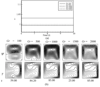
and 100≤Gr≤2000 as shown in [image:5.595.143.490.392.692.2]Figure 2(a). It is found that the flow is a steady-state solution for Dn=100 and 100≤Gr≤2000. To draw
Figure 2. (a) Time-dependent flow for Dn=100 and 100≤Gr≤2000; (b) Secondary flow
the contours for the stream lines of the secondary flow patterns
( )
ψ and temperature profiles (T), we use the increments ∆ =ψ
0.6 and ∆T = 0.25 respectively. The same increments of ψ and T are used for all the fig-ures in this study, unless specified. The right-hand side of each duct box of ψ and T is in the outside direction of the duct curvature. In the figures of the stream lines, solid lines(
ψ ≥0)
show that the secondary flow is in the counter clockwise direction while the dotted lines(
ψ <0)
in the clockwise direction. Similarly, in the fig-ures of the isotherms (temperature profiles), solid lines are those for T ≥0 and dotted ones for T < 0. Since the flow is steady-state, single contours of the secondary flow patterns and temperature profiles are shown in Figure 2(b), where it is seen that the unsteady flow is an asymmetric single- and two-vortex solution. It is found that asGr increases, the two-vortex solution ceases to be a single-vortex solution which covers the whole cross-section of the duct. We also investigated time-dependent solutions for Dn=500and 100≤Gr≤2000 and obtained same type of flow behavior as obtained for Dn=100. The results are shown in Figure 3, where we find that the unsteady flow is an asymmetric two-vortex steady-state solution.
Then, we investigated time-dependent solutions of λ for Dn=1000 and 100≤Gr≤2000. The results are shown in Figure 4(a). As seen in Figure 4(a), the time-dependent flow is a periodic solution for Gr=100 and
500
Gr= but steady-state solution for 1000≤Gr≤2000. In order to see the flow oscillations more clearly, we explicitly show time variations of λ for Gr=100 in Figure 4(b), where periodic flows are clearly observed. Contours of secondary flow patterns and temperature profiles are shown in Figure 4(c) for 23.45≤ ≤t 25.40. It is found that the periodic flow for Gr=100 oscillates between asymmetric four-vortex solution. Figure 5(a)
explicitly shows time evolution of λ for Dn=1000 and Gr=500, where it is seen that the flow oscillates pe-riodically. Corresponding secondary flow patterns and temperature profiles are shown in Figure 5(b) for 42.08≤ ≤t 42.30. As seen in Figure 5(b), the periodic oscillation for Gr=500 oscillates between asymme-tric two-vortex solutions. Since the unsteady flow is a steady-state solution for 100≤Gr≤2000, typical con-tours of the secondary flow patterns and temperature profiles are shown in Figure 5(c) for Gr = 1000, 1500 and 2000. In Figure 5(c), we see that the steady-state flow for Dn = 1000 and Gr = 1000, 1500 and 2000 are
Figure 3. (a) Time-dependent flow for Dn=500 and 100≤Gr≤2000; (b) Secondary flow
Figure 4. (a) Time-dependent flow for Dn=1000 and 100≤Gr≤2000; (b) time evolution of λ for Dn=1000 and 100
Gr= ; (c) secondary flow patterns (top) and temperature profiles (bottom) for Dn=1000 and Gr=100.
asymmetric two-vortex solution.
We then performed time evolution of λ for Dn = 1500 and 100≤Gr≤2000. The result is shown in Figure 6(a). As seen in Figure 6(a), the time-dependent flow for Dn=1500 is a steady-state solution for all 100≤Gr≤2000. Secondary flow patterns and temperature profiles, depicted in Figure 6(b) for Dn=1500, shows that the flow is an asymmetric two-vortex solution. The temperature profile is consistent with the second-ary vortices. The result of the time-dependent solution of λ for Dn=2000 and 100≤Gr≤2000 is shown in
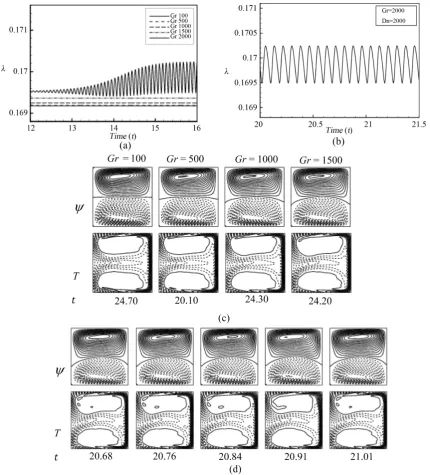
Figure 7(a). As seen in Figure 7(a), the time-dependent flow for Dn=2000 is a steady-state solution for 100≤Gr≤1500 but periodic oscillating flow for Gr=2000. The time-periodic flow for Gr=2000 is indi-vidually shown in Figure 7(b) for a clear view. Figure 7(c) shows typical contours of secondary flow patterns and temperature profiles for the steady-state solutions at 100≤Gr≤1500 and Figure 7(d) shows those for
2000
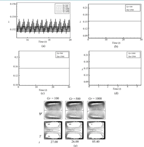
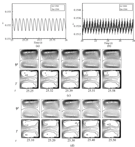
Gr= , for one period of oscillation at time 20.68≤ ≤t 21.01, and we find that both the time-periodic and steady-state solutions are asymmetric two-vortex solutions. Then we show the results of the time-dependent so-lutions for Dn=2500 and 100≤Gr≤2000 in Figure 8(a). As seen in Figure 8(a), the time-dependent flow for Dn=2500 is a steady-state solution for 100≤Gr≤1000 but periodic oscillating flow for Gr=1500 and multi-periodic (or transitional chaos) flow for Gr=2000. Figures 8(b)-(d) respectively show those of the time-dependent solutions for the steady-state solutions at Gr = 100, 500 and 1000. Since the flow is steady-state at Gr=100, 500 and 1000, a single contour of each of the secondary flow patterns and temperature profiles is shown inFigures 8(b)-(d) respectively. Figure 9(a) and Figure 9(b) respectively show time-dependent solu-tions for Gr=1500 and 2000 at Dn=2500. As seen in Figure 9(a) and Figure 9(b), the unsteady flow is a time-periodic for Gr=1500 but multi-periodic (sometimes called transitional chaos, (Mondal et al. [14]) for
2000.
(a)
(b)
[image:8.595.142.503.83.569.2](c)
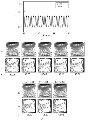
Figure 5. (a) Time-dependent flow for Dn=1000 and Gr = 500 at time 40≤ ≤t 46; (b) secondary flow patterns (top) and temperature profiles (bottom); (c) single contours of second-ary flow patterns (top) and temperature profiles (bottom) for Gr = 1000, 1500 and 2000 at
1000
Dn= .
flows are asymmetric two-vortex solution.
Figure 6. (a) Time-dependent flow for Dn=1500 and 100≤Gr≤2000; (b) contours of secondary flow patterns (top) and temperature profiles (bottom) for Dn=1500 and
100≤Gr≤2000.
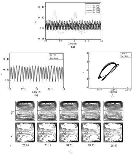
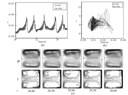
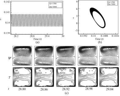
of secondary flow patterns and temperature profiles are shown in Figure 10(d), and it is found that the flow os-cillates between asymmetric two-vortex solutions. Then we explicitly show the result of the time-dependent flow for Dn=3000 and Gr = 500 in Figure 11(a). Then, to be sure whether the flow is periodic, mul-ti-periodic or chaotic, we draw the phase space of the time-dependent flow for Dn=3000 and Gr = 500 in
Figure 11(b) and see that the flow is a transitional chaos (Mondal [7]). Then we draw typical contours of sec-ondary flow patterns and temperature profiles for the transitional chaos at Dn=3000 and Gr = 500 in Figure 11(c). Figure 11(c) shows that the flow is an asymmetric two-vortex solution. Then we perform time-evolution of λ for Dn=3000 and Gr=1000, and presented in Figure 12(a). As seen in Figure 12(a), the flow oscil-lates multi-periodically. In order to see the characteristics of the multi-periodic oscillation, we draw the phase space of the time-dependent flow for Dn=3000 and Gr=1000 and presented in Figure 12(b). It is found that the unsteady flow creates irregular or multiple orbit which means the flow presented in Figure 12(a) is chaotic rather than multi-periodic. The chaotic behavior is clearly justified by Figure 12(b). Then we draw typ- ical contours of secondary flow patterns and temperature profiles for the chaotic oscillation at Dn=3000 and
1000
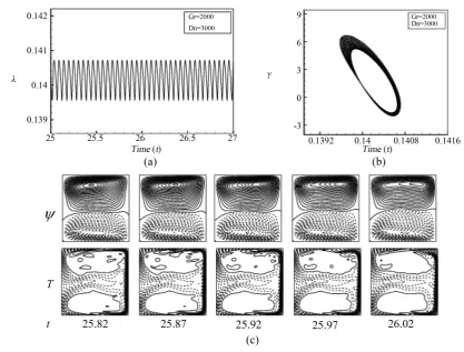
Gr= in Figure 12(c). As seen in Figure 12(c), the chaotic flow oscillates irregularly between the asym- metric two-vortex solutions. The results of the time-dependent flow for Gr=1500 and Gr=2000 at
3000
Dn= are shown in Figure 13(a) and Figure 14(a) respectively. As seen in Figure 13(a) and Figure 14(a), the unsteady flows at Gr=1500 and Gr=2000 are periodic solutions, which are well justified by drawing the phase-spaces as shown in Figure 13(b) and Figure 14(b) respectively. It is found that the two flows have nearly the same type of unsteady flow behavior. Typical contours of secondary flow patterns and temperature profiles for the periodic oscillations at Gr=1500 and Gr=2000 for Dn=3000 are shown in Figure 13(c)
entan-gled when the secondary vortices become stronger. In this regard, it should be worth mentioning that irregular oscillation of the non-isothermal and isothermal flows has been observed experimentally by Wang and Yang
[image:10.595.101.532.146.622.2][10] for a curved square duct flow and by Ligrani and Niver [22] for flow through a curved rectangular duct of large aspect ratio.
Figure 7. (a) Time-dependent flow for Dn=2000 and 100≤Gr≤2000; (b) time evolution of λfor Gr=2000; (c)
Figure 9. (a) Time-dependent flow for Dn=2500 and Gr=1500; (b) time evolution of λ for Dn=2500 and 2000
Gr= ; (c) contours of secondary flow patterns (top) and temperature profiles (bottom) for Gr=1500; (d) contours of
Figure 10. (a) Time-dependent flow for Dn=3000 and 100≤Gr≤2000; (b) time evolution of λ for Dn=3000 and 100
Figure 11. (a) Time-dependent flow for Dn=3000 and Gr=500; (b) phase space for Dn=3000 and 500
Gr= ; (c) secondary flow patterns (top) and temperature profiles (bottom) for Dn=3000 and Gr=500.
Figure 12. (a) Time-dependent flow for Dn=3000 and Gr=1000; (b) phase space for Dn=3000 and 1000
[image:14.595.113.521.447.602.2]Figure 12. (c) Secondary flow patterns (top) and temperature profiles (bottom) for Gr=1000.
Figure 13. (a) Time-dependent flow for Dn=3000 and Gr=1500; (b) phase space for Dn=3000 and 1000
[image:15.595.115.509.286.599.2]Figure 14. (a) Time-dependent flow for Dn=3000 and Gr=2000; (b) phase space for Dn=3000 and 2000
Gr= ; (c) secondary flow patterns (top) and temperature profiles (bottom) for Dn=3000 and Gr=2000.
4.2. Phase Diagram in the Dn-Gr Plane
Finally, the distribution of the time-dependent solutions, obtained by the time evolution calculations of the curved square duct flows, is shown in Figure 15 in the Dean number versus Grashof number (Dn-Gr) plane for 100≤Dn≤3000 and 100≤Gr≤2000, where the circle indicates steady-state solutions, the cross periodic (or multi-periodic) solutions and the triangle chaotic solutions. As seen in Figure 15, the unsteady flow is always a steady-state solution for any value of Gr in the range 100≤Gr≤2000, when 100≤Dn≤1500 except for
Dn = 1000. At Dn = 1000, the flow is periodic for Gr = 100 and 500 but steady-state otherwise. For Dn = 2000, the flow is periodic at Gr = 2000 but steady-state when Gr < 2000. As seen in Figure 15, the flow is also periodic/multi-periodic for Dn = 2500 at Gr = 1500 and 2000; for large Dean numbers, e.g. Dn = 3000, on the other hand, the unsteady flow changes in the scenario “periodic →chaotic →periodic”, if Gr in increased.
5. Conclusion
Figure 15.Distribution of the time-dependent solutions in the Dean number vs. Gra-shof number (Dn-Gr) plane for 100≤Dn≤3000 and 100≤Gr≤2000 ( Ο:
steady-state solution, ×: periodic solution, ∇: chaotic solution).
are also obtained, and it is found that periodic or multi-periodic solution oscillates between asymmetric two-, and four-vortex solutions, while for chaotic solution, there exist only asymmetric two-vortex solution. The tem-perature distribution is consistent with the secondary vortices and it is found that the temtem-perature distribution occurs significantly from the heated wall to the fluid as the secondary flow becomes stronger. The present study also shows that there is a strong interaction between the heating-induced buoyancy force and the centrifugal force in the curved passage which stimulates fluid mixing and thus results in thermal enhancement in the flow.
References
[1] Dean, W.R. (1927) Note on the Motion of Fluid in a Curved Pipe. Philosophical Magazine, 4, 208-223.
http://dx.doi.org/10.1080/14786440708564324
[2] Berger, S.A., Talbot, L. and Yao, L.S. (1983) Flow in Curved Pipes. Annual Review of Fluid Mechanics, 35, 461-512.
http://dx.doi.org/10.1146/annurev.fl.15.010183.002333
[3] Nandakumar, K. and Masliyah, J.H. (1986) Swirling Flow and Heat Transfer in Coiled and Twisted Pipes. Advances in Transport Process, 4, 49-112.
[4] Ito, H. (1987) Flow in Curved Pipes. JSME International Journal, 30, 543-552.
[5] Winters, K.H. (1987) A Bifurcation Study of Laminar Flow in a Curved Tube of Rectangular Cross-Section. Journal of Fluid Mechanics, 180, 343-369. http://dx.doi.org/10.1017/S0022112087001848
[6] Daskopoulos, P. and Lenhoff, A.M. (1989) Flow in Curved Ducts: Bifurcation Structure for Stationary Ducts. Journal of Fluid Mechanics, 203, 125-148. http://dx.doi.org/10.1017/S0022112089001400
[7] Mondal, R.N. (2006) Isothermal and Non-Isothermal Flows through Curved Duct with Square and Rectangular Cross- Section. Ph.D. Thesis,Department of Mechanical and Systems Engineering, Okayama University, Japan.
[8] Yanase, S. and Nishiyama, K. (1988) On the Bifurcation of Laminar Flows through a Curved Rectangular Tube. Jour-nal of the Physical Society of Japan, 57, 3790-3795. http://dx.doi.org/10.1143/JPSJ.57.3790
[9] Yanase, S., Kaga, Y. and Daikai, R. (2002) Laminar Flow through a Curved Rectangular Duct over a Wide Range of the Aspect Ratio. Fluid Dynamics Research, 31, 151-183. http://dx.doi.org/10.1016/S0169-5983(02)00103-X
[10] Wang, L. and Yang, T. (2005) Periodic Oscillation in Curved Duct Flows. Physica D, 200, 296-302.
http://dx.doi.org/10.1016/j.physd.2004.11.003
Advances in Heat Transfer, 38, 203-256. http://dx.doi.org/10.1016/s0065-2717(04)38004-4
[12] Yanase, S., Mondal, R.N., Kaga, Y. and Yamamoto, K. (2005) Transition from Steady to Chaotic States of Isothermal and Non-Isothermal Flows through a Curved Rectangular Duct.Journal of the Physical Society of Japan, 74, 345-358.
http://dx.doi.org/10.1143/JPSJ.74.345
[13] Yanase, S., Mondal, R.N. and Kaga, Y. (2005) Numerical Study of Non-Isothermal Flow with Convective Heat Trans-fer in a Curved Rectangular Duct. International Journal of Thermal Sciences, 44, 1047-1060.
http://dx.doi.org/10.1016/j.ijthermalsci.2005.03.013
[14] Mondal, R.N., Kaga, Y., Hyakutake, T. and Yanase, S. (2007) Bifurcation Diagram for Two-Dimensional Steady Flow and Unsteady Solutions in a Curved Square Duct. Fluid Dynamics Research, 39, 413-446.
http://dx.doi.org/10.1016/j.fluiddyn.2006.10.001
[15] Mondal, R.N., Uddin M.S. and Yanase, S. (2010) Numerical Prediction of Non-Isothermal Flow through a Curved Square Duct. International Journal of Fluid Mechanics Research, 37, 85-99.
http://dx.doi.org/10.1615/InterJFluidMechRes.v37.i1.60
[16] Chandratilleke, T.T. and Nursubyakto, S. (2003) Numerical Prediction of Secondary Flow and Convective Heat Transfer in Externally Heated Curved Rectangular Ducts. International Journal of Thermal Sciences, 42, 187-198.
http://dx.doi.org/10.1016/S1290-0729(02)00018-2
[17] Mondal, R.N., Kaga, Y., Hyakutake, T. and Yanase, S. (2006) Effects of Curvature and Convective Heat Transfer in Curved Square Duct Flows. Journal of Fluids Engineering, 128, 1013-1023. http://dx.doi.org/10.1115/1.2236131
[18] Norouzi, M., Kayhani, M.H., Nobari, M.R.H. and Karimi Demneh, M. (2009) Convective Heat Transfer of Viscoelas-tic Flow in a Curved Duct, World Academy of Science, Engineering and Technology, 32, 327-333.
[19] Norouzi, M., Kayhani, M.H., Shu, C. and Nobari, M.R.H. (2010) Flow of Second-Order Fluid in a Curved Duct with Square Cross-Section. Journal of Non-Newtonian Fluid Mechanics, 165, 323-339.
http://dx.doi.org/10.1016/j.jnnfm.2010.01.007
[20] Chandratilleke, T.T., Nadim, N. and Narayanaswamy, R. (2012) Vortex Structure-Based Analysis of Laminar Flow Behaviour and Thermal Characteristics in Curved Ducts. International Journal of Thermal Sciences, 59, 75-86.
http://dx.doi.org/10.1016/j.ijthermalsci.2012.04.014
[21] Gottlieb, D. and Orazag, S.A. (1977) Numerical Analysis of Spectral Methods. Society for Industrial and Applied Ma-thematics, Philadelphia.