http://dx.doi.org/10.4236/jcc.2015.311017
End
Point
Force
Control
of
a
Flexible
Timoshenko
Arm
Minoru Sasaki1, Kouki Nagaya1, Takahiro Endo2, Kojiro Matsushita1, Satoshi Ito1
1
Department of Mechanical Engineering, Gifu University, Gifu, Japan
2Department of Mechanical Engineering and Science, Graduate School of Engineering, Kyoto University, Kyoto,
Japan
Received September 2015
Abstract
Thispaperdiscussesaforcecontrolproblem foraflexibleTimoshenko arm.Theeffectofshear
deformationandtheeffectofrotaryinertiaareconsideredinTimoshenkobeamtheory.Mostof
the researchabout force control of the flexible arm is based on Euler Bernoulli beam theory.
ThereareafewresearchesaboutforcecontroloftheflexiblearmusingTimoshenkobeamtheory.
Theaimoftheforcecontrolistocontrolthecontactforceatthecontactpoint.Tosolvethisprob‐
lem,weproposeasimplecontrollerusingTimoshenkobeamtheory.Finally,wedescribesimula‐
tionresultsusinganumericalinversionofLaplacetransformcarriedouttoinvestigatethevalid‐
ityoftheproposedcontrollerfortheforcecontrolproblem.Theresultsofthetimeresponseshow
thetransversedisplacement,theangleofdeflection,thesliderposition,therotational angleand
thecontactforcetowardthedesiredtheirvalues.
Keywords
FlexibleArm,TimoshenkoBeamTheory,ForceControl,DistributedParameterSystemsControl,
LaplaceTransform
1.
Introduction
has a wider application area than the Euler-Bernoulli beam theory. So we discuss the force control problem for the flexible Timoshenko arm.
[image:2.595.208.415.548.704.2]2.
Equations
of
Motion
and
Boundary
Conditions
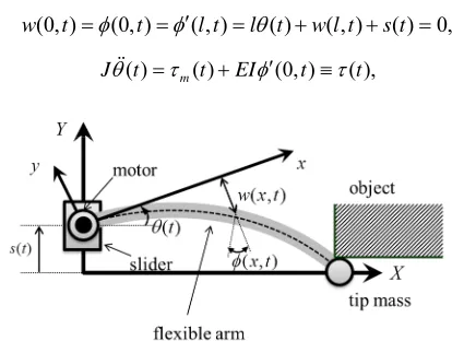
Figure 1 shows a constrained one-link flexible Timoshenko arm. One-end of the arm is clamped to control ac-tuators consisting of the rotational motor and the translational slider, and the other end has a concentrated tip mass m. The tip mass makes contact with the surface of an object. The flexible arm translates and rotates in the horizontal plane (the XY plane in Figure 1) by control actuators; it is not affected by the acceleration of grav-ity. The flexible arm, with length l, mass per unit length , mass moment of inertia I, cross sectional area
A, area moment of inertia I, Young’s modulus E, shear modulus G, and shear coefficient , satisfies the Timoshenko beam hypothesis.
In Figure 1, XY is an absolute coordinate system and xy is a local coordinate system, whose origin is fixed at the rotor of the rotational motor. In addition, xy translates with the slider and rotates with the rotor of the motor. Let J, m( )t , ( ) t , M , F ts( ), and ( )s t be the inertia moment of the motor, the torque
gener-ated by the motor at time t, the rotational angle of the motor, the mass of the slider, the force generated by the slider, and the translational position of the slider, respectively. Further, let ( , )w x t and ( , ) x t be the trans-verse displacement of the flexible arm at time t and spatial point x, and the rotation of the cross section due to bending deformation, respectively.
Since the tip mass makes contact with the surface of the object, we obtain the following geometric constraint: ( ) ( , ) ( ) 0
l t w l t s t
.
This constraint means that the Y-axis position of the tip mass is constrained on the surface of the object. The kinetic energy EK and the potential energy EP of the overall system are given by the following:
2 2 2
0
2 2
0
[ ( ) ( , ) ( )] d ( ) ( )
2 2 2
[ ( ) ( , )] d [ ( ) ( , ) ( )] ,
2 2
l K
l
J M
E x t w x t s t x t s t
I m
t x t x l t w l t s t
2 2
0[ ( , )] d 0[ ( , ) ( , )] d ,
2 2
l l
P
EI K
E
x t x
x t w x t xwhere K GA, a dot denotes the time derivative, and a prime denotes the partial derivative with respect to x. Here the virtual work is given by δW( ) t δ( )t F t( ) δs t( ).
Under the above preparation, we can obtain the following equations of motion by applying Hamilton’s princi-ple and Lagrange’s multiplier, and using the procedure described in [13]:
[ ( , )w x t x ( )t s t( )] K[ ( , )x t w x t( , )] 0,
(1)
[ ( , ) ( )] [ ( , ) ( , )] ( , ) 0,
I x t t K x t w x t EI x t (2) (0, ) (0, ) ( , ) ( ) ( , ) ( ) 0,
w t t l t l t w l t s t (3)
( ) m( ) (0, ) ( ),
Jt t EI t t (4)
( ) s( ) (0, ) ( ),
M s t F t Kw t F t (5) with the algebraic relation
( )t K w l t[ ( , ) ( , )],l t
(6) where ( ) t is Lagrange’s multiplier and is equivalent to the contact force, i.e., the shear force at the tip of the flexible arm, which arises in the direction along the normal vector of the constraint surface.
The aim of this paper is to control the contact force at the tip of the flexible arm. In other words, the control objective is to construct a boundary controller satisfying
( ) , ( , ) 0, ( , ) 0,
( ) 0, ( ) 0,
d
t w x t x t
t s t
(7)
where d is the constant desired contact force. At the desired equilibrium point
(( )t d, ( , )w x t ( , )x t ( )t s t( ) 0 ), w x t( , ) and ( , )x t become the function of the variable x, and ( )t
and ( )s t become constant. Thus, we describe them as w xd( ), d( )x , d, and sd, respectively. By
sub-stituting these into (1)-(6), we obtain:
2
2
1
( ) , ( ) ,
2 6 2
1
, 3
d
d d d
d d d
x
lx x x
w x x x l
K EI EI EI
l
l s l
K EI
(8)
In these relations, w xd( ), d( )x , d, and sd mean a static transverse displacement, a static rotation of the
cross section of the flexible arm, a static angle of the motor, and a static position of the slider in the case where the contact force is converged to the desired value, respectively. Furthermore, d and sd are coupled through
d
, and thus we cannot set the desired angle d and the desired position sd independently.
Based on these results, we set the control objective as follows: to construct a controller accomplishing:
( , ) ( ), ( , ) 0,
( , ) ( ), ( , ) 0,
( ) , ( ) 0, ( ) , ( ) 0.
d
d
d d
w x t w x w x t
x t x x t
t t s t s s t
(9)
For this purpose, we propose the following controller:
1 2 3 4
( ) [ (0, ) d(0)] (0, ) [ ( ) d] ( ),
F t k K w t w k Kw t k s t s k s t (10)
5 6 7 8
( )t k EI[ (0, )t d(0)] k EI (0, )t k[ ( )t d] k ( ),t
(11) where feedback gain ki, i1, ,8 , is a positive constant. In these controllers, (10) is the controller for the
slider and (11) is the controller for the motor. In (10), the first and second terms are for the control: ( , ) d( )
w x t w x and ( , )w x t 0, and the third and the forth terms are for the position control: ( )s t sd and
( ) 0
s t . On the other hand, in (11), the first and second terms are for the control of the rotation of the cross section: ( , ) x t d( )x and ( , )x t 0, and the third and the forth terms are for ( ) t d and ( )t 0.
Here, note that if we use the strain gauge, rotary encoder, and speed reference type servo amplifier of the motor and the slider, we can easily implement the controller.
3.
Laplace
Transform
of
the
Equation
of
Motion
Taking the Laplace transform of (1)-(11), we can get
2 , , , 2 0
s w x s K x s K w x s s x s S s (12)
2
,
,
, 2
0s IK x s Kw x s EI x s s I s (13)
0, 0
0,s 0 (15)
l s, 0 (16)
,
0l s w l s S s (17)
2 (0, ) ( )
m
s J s s EI s s (18)
2 (0, )
s
s MS s F s Kw s F s (19)
1 2
3 4
1
31
0, ( d 0 d)
F s k sk Kw' s k sk S s k Kw ' k S
s
(20)
5 6
7 8
5
71
0, ( d 0 d)
s k sk EI s k sk s k EI k
s
(21)
Finally we get w
0,s and
0,s as follows:
2 2 2
4 3 7 8
2 2
4 3 7 8
2 2 2 2 2 2 2 2
3 2
8 4 2 6 3 4 8 7
2 2
3 4 8 7 1 6 2 5 3 8 4 7
1 1
0, ( 2 2 1
4 *( 1 *( 4 2 ( 2 1 1 2 2 2
w s F s F s
K s sk s k k sk s E I
sk s k k sk s
s E I KE s I K I K s I s EI I K
k k EI I K s E K k k k k k k I
I K k J k k Mk s E k k k k K k k k k
23 8 4 7 3 7 1 5 3 7
2 2 2 2 2 2 2 2
2 2
4 3 7 8
2 2 2 2 2 2 2 2
3 2
8 4 2
1
) 2 ( ) ))
2 1 * 4 2 2 1 * 4 2 ( 2 I
KI k k k k s E k k K k k I KI k k
KEI s EI KsI s E I KE s I K I K s I s
sk s k k sk s
s E I KE s I K I K s I s EI I K
k k EI I K s E K k
6 3 4 8 7
2 2
3 4 8 7 1 6 2 5 3 8 4 7
2
3 8 4 7 3 7 1 5 3 7
2 2
1 2 7 8
2 2 2 2 2 2 2 2
1 2 7
1 1
2
2 2
1
) 2 ( ) ))
2
2 ( 3 2 1 4 *
1 4
2
k k k k k I
I K k k k k s E k k k k K k k k k I
KI k k k k s E k k K k k I KI k k
EIK s F s F s F s F s k sk k sk s
s E I KE s I K I K s I
s k sk k
2 2 2
8
2
1 3 2 5 7
8 1 3 1 2 5 7 7 1 3
* 2
* 1 2 3 4 2( (
) ) ) 0,
d d d d
d d d d d d
sk s EI I K s K
F s F s F s F s k k S s k k l k K
k k k S s k k k l k K k k k S K
5 6
2
7 8
2 2 2 2 2 2 2 2
2 2 2 2 2 2 2 2
5 6
5 7
1 1
0, ( 2 2 1
2
1
* 4 2 4 3
2
1
* 4
2
2 ( d d)) 1 2 3
s s F s F s k sk
Ks k sk s
KEI s EI KsI s E I KE s I K I K s I s s F s F s
k sk KEI s EI KsI s E I KE s I K I K s I s
K k l k F s F s F
s F4
s 0,(23)
where the constants F1
s , 2F
s , 3F
s and 4( )F s can be determined using the boundary conditions.4.
Numerical
Simulation
Results
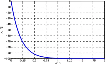
Numerical inversion of Laplace transform is used to obtain the results in the time domain. The computation of the inverse Laplace transform is based on the paper of T. Hosono [12]. In the computer simulation study, we consider a typical arm whose parameters are given in the Table 1. To investigate the validity of the proposed controller, we considered the step responses of the desired contact force, d 100 N, and the desired posi-tion of the slider, sd 0.1 m. Here, note that d 100 means that the flexible arm pushed the surface of the
environment by the force of 100 N. Figures 2-6 show the time response of the transverse displacement, the an-gle of deflection, the slider position, the rotational anan-gle and the contact force with adequate feedback gains
1 5 1
k k , k2k60.2, k3k716, k4k88 using try and error method. The desired value of wd,
d
, d are
0 0.25 0.5 0.75 1 1.25 1.5 1.75 2
-5 -4.5 -4 -3.5 -3 -2.5 -2 -1.5 -1 -0.5
0x 10 -3
w[
m
]
t[s]
Figure 2. Time response of transverse displacement of the arm.
0 0.25 0.5 0.75 1 1.25 1.5 1.75 2
-7 -6 -5 -4 -3 -2 -1
0x 10 -3
t[s]
φ[
ra
d
]
0 0.25 0.5 0.75 1 1.25 1.5 1.75 2 -0.02
0 0.02 0.04 0.06 0.08 0.1 0.12
t[s]
S[
m
[image:6.595.217.406.87.216.2]]
Figure 4. Time response of the slider position.
0 0.25 0.5 0.75 1 1.25 1.5 1.75 2 -0.1
-0.08 -0.06 -0.04 -0.02 0 0.02
t[s]
θ[
ra
[image:6.595.218.407.248.376.2]d]
Figure 5. Time response of rotational angle.
0 0.25 0.5 0.75 1 1.25 1.5 1.75 2
-100 -90 -80 -70 -60 -50 -40 -30 -20 -10 0
t[s]
λ[
N
]
Figure 6. Time response of the contact force. Table 1. System parameters.
Length l 1.0 [m]
Mass per unit length 2.73 [kg/m]
Mass moment of inertia I 2.79e (−4) [kgm]
Cross sectional area A 3.5e (−4) [m4]
Area moment of inertia I 3.57e (−8) [m4]
Young’s modulus E 2.00e11 [Pa]
Shear modulus G 7.69e10 [Pa]
Shear coefficient 5/6
Desired contact force d −100 [N]
[image:6.595.220.407.409.523.2] [image:6.595.107.538.570.719.2]
3
3
7.00 10 [ ]
4.67 10 [ ]
0.0953[ ]
d
d
d
x rad
w x m
rad
(24)
It can be seen that the transverse displacement, the angle of deflection, the slider position, the rotational angle and the contact force toward the desired their values. With the adequate feedback gains there are no residual vi-brations and no over shoot.
5.
Conclusion
A contact-force control problem with regards to a constrained one-link flexible Timoshenko arm was described. The equations of motion and the boundary conditions of the overall system were derived. To solve the contact force control problem of such a system, we have proposed a simple controller, which is easy to implement. Sev-eral numerical simulations using a numerical inversion of Laplace transform were carried out. The simulation results showed the validity of the proposed controller for the contact-force control problem with no residual vi-brations and no overshoot.
References
[1] Yuan, K. and Hu, C.-M. (1996) Nonlinear Modeling and Partial Linearizing Control of a Slewing Timoshenko-Beam.
Trans. ASME Journal of Dynamic Systems, Measurement, and Control, 118, 75-83.
[2] Tadi, M. (1997) Comparison of Two Finite-Element Schemes for Feedback Control of a Timoshenko Beam. Proceed-ings of the ASME Dynamic Systems and Control Division, 61, 587-596.
[3] White, M.H.D. and Heppler, G.R. (1996) Vibration of a Rotating Timoshenko Beam. Trans. ASME Journal of
Vibra-tion and Acoustic, 118, 606-
[4] Sasaki, M., Ueda, T., Inoue, Y. and Book, W.J. (2012) Passivity-Based Control of Rotational and Translational Ti-moshenko Arms. Advances in Acoustics and Vibration, 2012, Article ID: 174816.
[5] Morgül, Ö. (1992) Dynamic Boundary Control of the Timoshenko Beam. Automatica, 28, 1255-1260.
[6] Oguamanam, D.C.D. and Heppler, G.R. (1996) The Effect of Rotating Speed on the Flexural Vibration of a Ti-moshenko Beam. Proc. of the 1996 IEEE International Conference on Robotics and Automation, 2438-2443.
[7] Zhang, F., Dawson, D.M., de Queiroz, M.S. and Vedagarbha, P. (1997) Boundary Control of the Timoshenko Beam with Free-End Mass/Inertial Dynamics. Proc. of the 36th IEEE Conference on Decision & Control, 245-250.
[8] Taylor, S.W. and Yau, S.C.B. (2003) Boundary Control of a Rotating Timoshenko Beam. ANZIAM J., 44, E143-E184.
[9] Rastgoftar, H., Mahmoodi, M., Eghtesad, M. and Kazemi, M. (2008) Stability Analysis of a Flexible Two-Link Ti-moshenko Manipulator Using Boundary Control Method. Proc. of ASME 2008 International Mechanical Engineering Congress and Exposition, 409-415.
[10] Grobbelaar-Van Dalsen, M. (2010) Uniform Stability for the Timoshenko Beam with Tip Load. J. Math. Anal. Appl.,
361, 392-400
[11] Han, Z.J. and Xu, G.Q. (2011) Dynamical Behavior of a Hybrid System of Nonhomogeneous Timoshenko Beam with
Partial Non-Collocated Inputs. J. Dyn. Control Syst., 17, 77-121.
[12] Hosono, T. (1981) Numerical Inversion of Laplace Transform and Some Application to Wave Optics. Radio Science,
16, 1015.
[13] Endo, T., Matsuno, F. and Kawasaki, H. (2014) Force Control and Exponential Stabilisation of One-Link Flexible Arm.