Complex Dynamics of Sine Function using Jungck Ishikawa Iterates

(1)

Complex Dynamics of Sine Function using Jungck

Ishikawa Iterates

Suman Pant

Research Scholar G. B. Pant Eng. College,

Pauri Garhwal

Yashwant S.Chauhan,

Ph.D

Assistant Professor G. B. Pant Eng. College,

Pauri Garhwal

Priti Dimri,

Ph.D

Asso. Professor and Head G. B. Pant Eng. College,

Pauri Garhwal

ABSTRACT

The dynamics of transcendental function is one of emerging and interesting field of research nowadays. We introduce in this paper the complex dynamics of sine function of the type {sin (zn ) – z + c = 0} and applied Jungck Ishikawa iteration to generate Relative Superior Mandelbrot set and Relative Superior Julia set. In order to solve this function by Jungck – type iterative schemes, we write it in the form of Sz = Tz, where the function T, S are defined as Tz = sin ( zn ) +c and Sz= z. Only mathematical explanations are derived by applying Jungck Ishikawa Iteration for transcendental

function in the literature but in this paper we have generated relative Mandelbrot sets and Relative Julia sets.

Keywords

Complex dynamics, Relative Superior Mandelbrot set, Relative Julia set, Jungck Ishikawa Iteration

1. INTRODUCTION

The study of dynamical behavior of the transcendental functions was initiated by Fatou [12]. For transcendental function, points with unbounded orbits are not in Fatou sets but they must lie in Julia sets. Attractive points of a function have a basin of attraction, which may be disconnected. A point z in Julia for sine function has an orbit that satisfies | Imz |>=50.

The iteration of complex analytic function (f) decompose the complex plane into two disjoint sets

1. Stable Fatou sets on which the iterations are well behaved. 2. Julia sets on which the map is chaotic.

In this past literature the sine function was considered of the following forms:

(i) sin (zn) + c = 0 (ii)(sin z + c)n = 0

We are using in our paper sine function of the type sin(zn) – z + c = 0 where n



2 and applied Jungck Ishikawa iterates to develop fractal images of this transcendental function. Escape criteria of polynomials are used to generate Relative Superior Mandelbrot Sets and Relative Superior Julia Sets. Our results are different from existing results in literature.

2. PRELIMINARIES

The process of generating fractal images from z sin (zn ) – z + c is similar to the one employed for the

self-squared function [17]. Briefly, this process consists of iterating this function up to N times.

Starting from a value z0 we obtain z1, z2, z3 , z4 ... by applying

the transformation z sin (zn ) – z + c

2.1 Ishikawa Iteration [2]

Let X is a subset of real or complex numbers and T: X→ X for x0∈ X, we have the sequences {xn} and {yn} in X in the

following manner:

x n+1 = αn T y n + (1- α n ) x n

y n = βn T x n + (1- β n ) x n

where 0 ≤ βn ≥ 1 and 0 ≤ αn ≥ 1 and αn & βn both convergent to non zero number.

2.2 Definition [1]

The sequences {xn} and {yn} constructed above is called

Ishikawa sequences of iteration or relative superior sequences of iterates. We denote it by (x0, α n , β n ,t) .Notice that RSO

(x0, α n , β n ,t) with β n = 1 is RSO(x0, α n ,t) i.e. Mann’s orbit

and if we place α n = β n =1 then RSO (x0, α n , β n ,t) reduces

to O (x0, t ) .We remark that Ishikawa orbit RSO(x0, α n , β n ,t)

with β n = 1/2 is Relative superior orbit. Now we define

Julia set for function with respect to Ishikawa iterates. We call them as Relative Superior Julia sets.

2.3 Definition [1]

The set of points SK whose orbits are bounded under Relative superior iteration of function Q (z) is called Relative Superior Julia sets. Relative Superior Julia set of Q is a boundary of Julia set RSK.

2.4 Jungck Ishikawa Iteration [2]

Let(X, ║.║) be a Banach space and Y an arbitrary set. Let S, T: Y→X be two non self-mappings such that T(Y) S(Y), S(Y) is a complete subspace of X and S is injective. Then for xo ∈Y, define the sequence {S x n }iteratively by

S x n+1 = α n T y n + (1- α n ) S x n

S y n = β n T x n + (1- β n ) S x n

where 0 ≤ βn ≥ 1 and 0 ≤ αn ≥ 1 and αn & βn both convergent

(2)

3. FIXED POINTS

3.1 Fixed points of quadratic function

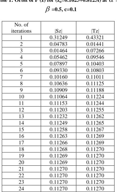
Table 1: Orbit of F (z) for (zo=0.1625+0.8125i) at



=0.5,



=0.5, c=0.1

No. of

iterations |Sz| |Tz|

1 0.31249 0.43321

2 0.04783 0.01441

3 0.01464 0.07266

4 0.05462 0.09546

5 0.07897 0.10403

6 0.09330 0.10803

7 0.10160 0.11011

8 0.10636 0.11125

9 0.10909 0.11188

10 0.11064 0.11224

11 0.11153 0.11244

12 0.11203 0.11255

13 0.11232 0.11262

14 0.11249 0.11265

15 0.11258 0.11267

16 0.11263 0.11269

17 0.11266 0.11269

18 0.11268 0.11270

19 0.11269 0.11270

20 0.11269 0.11270

21 0.11270 0.11270

22 0.11270 0.11270

23 0.11270 0.11270

24 0.11270 0.11270

Here we observe that the value converges to a fixed point after 21 iterations.

0 5 10 15 20 25 30

[image:2.595.335.531.66.307.2]

0 0.02 0.04 0.06 0.08 0.1 0.12 0.14 0.16 0.18

Figure 1: Orbit of F(x) for (zo = 0.1625+0.8125i) at



=0.5,

[image:2.595.67.260.105.422.2]



=0.5, c=0.1

Table 2: Orbit of F (z) for (z0=-2.55+0.375i) at



=0.3,



=0.7, c=0.1

No. of

1 0.27560 2.46585

2 0.74621 1.37485

3 0.72702 0.55117

4 0.48395 0.17341

5 0.15496 0.02913

6 0.07996 0.09661

7 0.09854 0.10888

8 0.10783 0.11155

9 0.1111 0.11233

10 0.11218 0.11258

11 0.11253 0.11266

12 0.11265 0.11269

13 0.11268 0.11270

14 0.11270 0.11270

15 0.11270 0.11270

16 0.11270 0.11270

17 0.11270 0.11270

18 0.11270 0.11270

19 0.11270 0.11270

20 0.11270 0.11270

Here we observe that the value converges to a fixed point after 14 iterations

0 5 10 15 20 25 30 35 40 45 50

-3 -2.5 -2 -1.5 -1 -0.5 0 0.5

Figure 2. Orbit of F(x) for (zo=-2.55+0.375i) at



=0.3,

[image:2.595.330.514.341.501.2]



=0.7, c=0.1

Table 3: Orbit of F (z) for (zo=-0.1375-0.0625i) at



=0.5,



=0.8, c=0.1 No. of

140 0.11269 0.1127

141 0.11269 0.1127

142 0.11269 0.1127

143 0.11269 0.1127

144 0.11269 0.1127

145 0.11269 0.1127

146 0.11270 0.1127

147 0.11270 0.1127

148 0.11270 0.1127

149 0.11270 0.1127

150 0.11270 0.1127

[image:2.595.68.268.476.633.2]

(3)

0 5 10 15 20 25 30 -0.2

-0.15 -0.1 -0.05 0 0.05 0.1 0.15

Figure 3: Orbit of F (z) for (zo=-0.1375-0.0625i) at



=0.5,



=0.8, c=0.1

[image:3.595.330.529.70.435.2]

3.2 Fixed points of cubic function

Table 1: Orbit of F (z) for (zo=-0.6125+0i) at



=0.5,



=0.5, c=0.1

No. of

1 0.09375 0.08144

2 0.09884 0.10013

3 0.10053 0.10098

4 0.10093 0.10103

5 0.10101 0.10103

6 0.10103 0.10103

7 0.10103 0.10103

8 0.10103 0.10103

9 0.10103 0.10103

10 0.10103 0.10103

0 5 10 15 20 25 30

-0.7 -0.6 -0.5 -0.4 -0.3 -0.2 -0.1 0 0.1 0.2

Figure 1 Orbit of F (z) for (zo=-0.6125+0i) at



=0.5,

[image:3.595.66.259.340.488.2]



=0.5, c=0.1

Table 2: Orbit of F (z) for (zo=-0.2625+1.10625i) at



=0.3,



=0.7, c=0.1

0 5 10 15 20 25 30

-0.3 -0.25 -0.2 -0.15 -0.1 -0.05 0 0.05 0.1 0.15

Figure 2: Orbit of F (z) for (zo=-0.2625+1.10625i) at



=0.3,



=0.7, c=0.1 No. of

1 0.02500 0.04437

2 0.06846 0.03949

3 0.08382 0.05806

4 0.08882 0.08958

5 0.09342 0.09785

6 0.09676 0.10012

7 0.09875 0.10076

8 0.09984 0.10094

9 0.10042 0.10100

10 0.10072 0.10102

11 0.10087 0.10103

12 0.10095 0.10103

13 0.10099 0.10103

14 0.10101 0.10103

15 0.10102 0.10103

16 0.10103 0.10103

17 0.10103 0.10103

18 0.10103 0.10103

19 0.10103 0.10103

[image:3.595.73.264.553.697.2]

(4)

Table 3: Orbit of F (z) for (zo = 0.1875+0.175i) at



=0.5,



=0.8, c=0.1

No. of

1 1.10625 -0.73928

2 0.13639 -0.1472

3 0.12193 0.02143

4 0.11184 0.07494

5 0.1062 0.09209

6 0.10355 0.09787

7 0.10232 0.0999

8 0.10172 0.10063

9 0.10142 0.10089

10 0.10125 0.10098

11 0.10116 0.10101

12 0.10111 0.10103

13 0.10108 0.10103

14 0.10106 0.10103

15 0.10105 0.10103

16 0.10104 0.10103

17 0.10104 0.10103

18 0.10103 0.10103

19 0.10103 0.10103

20 0.10103 0.10103

0 5 10 15 20 25 30

[image:4.595.326.518.92.322.2]

0.1 0.11 0.12 0.13 0.14 0.15 0.16 0.17 0.18 0.19

Figure 3: Orbit of F (z) for (zo = 0.1875+0.175i) at



=0.5,



=0.8, c=0.1

3.3 Fixed points of biquadratic function

Table 1: Orbit of F (z) for (zo= 0.0375+0.625i) at



=0.5,



=0.5, c=0.1

No. of

1 0.00625 0.29254

2 0.07642 0.09973

3 0.09532 0.10004

4 0.09914 0.10009

5 0.09991 0.1001

6 0.10006 0.1001

7 0.10009 0.1001

8 0.1001 0.1001

9 0.1001 0.1001

10 0.1001 0.1001

0 5 10 15 20 25 30

[image:4.595.62.271.94.450.2]

0.03 0.04 0.05 0.06 0.07 0.08 0.09 0.1 0.11

Figure 1: Orbit of F (z) for (zo= 0.0375+0.625i) at



=0.5,

[image:4.595.329.520.377.529.2]



=0.5, c=0.1

Table 2: Orbit of F (z) for (zo= 0.1-0.3i) at



=0.3,



=0.7,

c=0.1

No. of

1 0.06875 1.46516

2 0.48917 0.15118

3 0.20888 0.08937

4 0.05448 0.09998

5 0.02276 0.10000

6 0.06138 0.09999

7 0.08071 0.10003

8 0.09038 0.10006

9 0.09523 0.10008

10 0.09766 0.10009

11 0.09888 0.10010

(5)

13 0.09979 0.10010

14 0.09995 0.10010

15 0.10002 0.10010

16 0.10006 0.10010

17 0.10008 0.10010

18 0.10009 0.10010

19 0.10010 0.10010

20 0.10010 0.10010

0 5 10 15 20 25 30

0.0999 0.0999 0.1 0.1 0.1001 0.1001 0.1002

Figure 2: Orbit of F (z) for (zo= 0.1-0.3i) at



=0.3,

[image:5.595.62.246.72.160.2]



=0.7, c=0.1

Table 3: Orbit of F (z) for (zo = 0.2375+0i) at



=0.5,



=0.8, c=0.1

No. of

1 0.26875 0.81993

2 0.04699 0.09997

3 0.06819 0.09994

4 0.08093 0.10000

5 0.08858 0.10004

6 0.09318 0.10007

7 0.09594 0.10008

8 0.09760 0.10009

9 0.09860 0.10009

10 0.09920 0.10010

11 0.09956 0.10010

12 0.09978 0.10010

13 0.09991 0.10010

14 0.09998 0.10010

15 0.10003 0.10010

16 0.10006 0.10010

17 0.10007 0.10010

18 0.10009 0.10010

19 0.10009 0.10010

20 0.10009 0.10010

21 0.10010 0.10010

22 0.10010 0.10010

23 0.10010 0.10010

24 0.10010 0.10010

25 0.10010 0.10010

0 5 10 15 20 25 30

0.1 0.12 0.14 0.16 0.18 0.2 0.22 0.24

Figure 3: Orbit of F (z) for (zo= 0.2375+0i) at



=0.5,



=0.8, c=0.1

4. GEOMETRY OF RELATIVE

SUPERIOR MANDELBROT SETS AND

RELATIVE SUPERIOR JULIA SETS

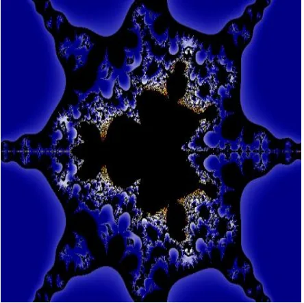
Relative Superior Mandelbrot Sets

 In case of quadratic function, the central body is divided into two parts. It is seen that the body is symmetric along the real axis only. Secondary lobes are very small initially for



= 1,



=1. As the value is changed to



=0.3



=0.7, the central body is divided into four parts but the middle part is quite larger in comparison to the head and tail.

Secondary lobes seem to appear larger than initial stage.  In case of cubic function, the central body is divided into

two equal parts, each part have one major secondary lobe and many minor secondary lobes. It is seen that the body is symmetric along the both axes. For



=0.3,



=0.7, the size of the major secondary lobes start enlarging and also a tiny bulb seems to occur along the real axis.  In case of biquadratic function, the central body is

divided into three parts, each part having one major secondary bulb along with large number of minor secondary bulbs. It is seen that the body is symmetric along the real axis only. For



=0.3,



=0.7, the two of the major secondary lobes are same in size but one of them grows larger in size and undergoes bifurcation along the real axis.

Relative Superior Julia Sets

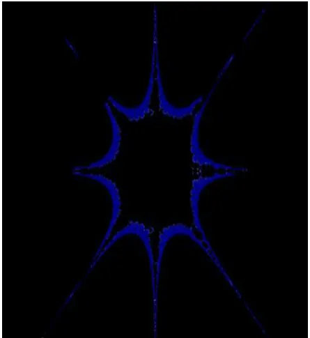
[image:5.595.331.513.178.320.2]

(6)

wings. These sets are symmetric along both the axes i.e. along real and imaginary axis.

 The Relative Superior Julia Sets for quadratic function is divided into four wings having black central body. These sets are symmetric along both the axes.

 The Relative Superior Julia Sets for Cubic function is divided into six wings having reflectional and rotational symmetry, along with a larger black region.

 The Relative Superior Julia Sets for biquadratic function is divided into eight wings possessing the reflectional and rotational symmetry, along with a larger escape region as compared to quadratic and cubic function.

 It is also observed from the graphical study of fixed points of Relative Superior Julia Sets that the convergence for





=0.3,



=0.7 is quite fast for all polynomials in comparison to the convergence for



=0.5,



= 0.8.

5. GENERATION OF RELATIVE

SUPERIOR MANDELBROT SETS

We generated the Relative Superior Mandelbrot sets. We present here some beautiful filled Relative Superior Mandelbrot sets for quadratic, cubic and biquadratic function.

[image:6.595.315.543.72.314.2]

6.1 Relative Superior Mandelbrot sets for

Quadratic function

Figure 1: Relative Superior Mandelbrot Set for

[image:6.595.314.538.334.599.2]



=



=0.5 & c = -0.1625+0.8125i



=0.3,



=0.7, c=-2.55+0.375i



=0.5,



=0.8, c=-0.1375-0.0625i

[image:6.595.55.277.415.645.2]

(7)

[image:7.595.54.266.69.302.2] [image:7.595.316.538.72.303.2]

[image:7.595.54.273.346.592.2]



=



=0.5, c=-0.6125+0i



=0.3,



=0.7, c = -0.2625+1.10625i



=0.5,



=0.8, c = 0.1875+0.175i

[image:7.595.315.537.382.603.2]

6.3 Relative Superior Mandelbrot sets for

biquadratic function



=0.5,

(8)

[image:8.595.54.274.68.307.2] [image:8.595.314.536.85.323.2]



=0.3,



=0.7, c = 0.1-0.3i



=0.5,



=0.8, c = 0.2375+0i

6. GENERATION OF RELATIVE

SUPERIOR JULIA SETS

We generated the Relative Superior Julia sets. We have presented here some beautiful filled Relative Superior Julia sets for quadratic, cubic and biquadratic function.

5.1 Relative Superior Julia sets for

[image:8.595.57.278.357.587.2]

Quadratic function

Figure 1: Relative Superior Julia Set for



=



=0.5, c=0.1625+0.8125i

[image:8.595.314.531.370.614.2]

(9)

[image:9.595.54.271.71.314.2] [image:9.595.315.533.72.315.2]



=0.5,



=0.8, c=-0.1375-0.0625i

5.2 Relative Superior Julia Sets for Cubic

function

[image:9.595.314.534.359.605.2]



=



=0.5, c=-0.612+0i

[image:9.595.54.271.391.637.2]



=0.3,



=0.7, c = -0.2625+1.10625i



=0.5,



=0.8, c = 0.1875+0.175i

(10)

[image:10.595.314.537.71.314.2] [image:10.595.54.266.72.316.2]



= 0.5,



= 0.5, c=0.0375+0.625i



= 0.3,



= 0.7, c=0.1-0.3i



= 0.5,



= 0.8, c=0.2375+0i

7. CONCLUSION

In this paper we studied the sine function which is one of the members of transcendental family. The fixed point 0 for S (z) = sin (zn ) – z + c = 0 also satisfies S’ (0) = 1. Orbits on the real axis tend to 0 while orbits on the imaginary axis tend to infinity. Relative Superior Julia Sets for the transcendental function sin (z) appears to follow law of having 2n wings. The surrounding region of the Mandelbrot set appears to be an invariant Cantor set in the form of curve or “hair” that extends to



. The orbit of any point on hair tends to infinity under iteration. Here the geometry of hairs is quite similar to that of exponential family and hence showed the property of transcendental function. The region filled up with large number of escaping points represents Julia set plane.

8. REFERENCES

[1] Suman Joshi, Dr.Yashwant Singh Chauhan and Dr. Ashish Negi, “New Julia and Mandelbrot Sets for Jungck Ishikawa Iterates” International Journal of Computer Trends and Technology (IJCTT), vol.9, no.5, pp.209-216, 2014.

[2] Suman Joshi, Dr.Yashwant Singh Chauhan and Dr.Priti Dimri ,“Complex Dynamics of Multibrot Sets for Jungck Ishikawa Iteration” International Journal of Research in Computer Applications and Robotics (IJRCAR), vol. 2, no. 4, pp. 12-22, 2014.

[3] M.O.Olatinwo, “Some stability and strong convergence results for the Jungck-Ishikawa iteration process,”Creative Mathematics and Informatics, vol. 17, pp. 33-42, 2008.

[4] R. Chugh and V. Kumar, “Strong Convergence and Stability results for Jungck-SP iterative scheme, International Journal of Computer Applications, vol. 36,no. 12, 2011.

[image:10.595.53.277.361.602.2]

(11)

[6] G. Julia, “Sur 1’ iteration des functions rationnelles”, JMath Pure Appli. 8 (1918), 737-747

[7] B. B. Mandelbrot, The Fractal Geometry of Nature, W. H.Freeman, New York, 1983.

[8] Eike Lau and Dierk Schleicher, “Symmetries of fractals revisited.” Math. Intelligencer (18) (1) (1996), 45-51.MR1381579 Zbl 0847.30018.

[9] J. Milnor, “Dynamics in one complex variable; Introductory lectures”, Vieweg (1999).

[10] Shizuo Nakane, and Dierk Schleicher, “Non-local connectivity of the tricorn and multicorns”, Dynamical systems and chaos (1) (Hachioji, 1994), 200-203, World Sci. Publ., River Edge, NJ, 1995. MR1479931.

[11] Rajeshri Rana, Yashwant S Chauhan and Ashish Negi.Article: Non Linear Dynamics of Ishikawa

Iteration. International Journal of Computer Applications 7(13):43–49, October 2010. Published By Foundation of Computer Science.ISBN: 978-93-80746-97-5.

[12] Ashish Negi, “Generation of Fractals and Applications”, Thesis, Gurukul Kangri Vishwvidyalaya, (2005). [13] M.O.Osilike, “Stability results for Ishikawa fixed point

iteration procedure”, Indian Journal of Pure and Appl. Math., 26(1995), 937-945.

[14] A. G. D. Philip: “Wrapped midgets in the Mandelbrot set”, Computer and Graphics 18 (1994), no. 2, 239-248. [15] Shizuo Nakane, and Dierk Schleicher, “On multicorns