Munich Personal RePEc Archive
Optimal Technology and Development
Moscoso Boedo, Hernan
University of Virginia
September 2006
Online at
https://mpra.ub.uni-muenchen.de/1644/
Optimal Technology and Development
∗
Hernan J. Moscoso Boedo
†University of Virginia
September 22nd 2006
Abstract
Skill intensive technologies seem to be adopted by rich countries rather than poor
ones. Related to that observation, the ratio of wages of skilled to unskilled workers
-the skill premium - shows two important features over time and across countries. In
the US the skill premium decreased during the first half of the 20th century and it
increased after 1950, evolving according to a U shaped pattern. On the other hand,
the same measure across countries around 1990 is hump shaped when countries are
ordered by GDP per worker.
By modeling the decisions for factor accumulation and technology adoption, this
paper gives a systematic explanation as to why we see ever more skill intensive
technolo-gies being adopted both over time in the US and across countries. The model developed
here endogenously generates predictions for the skill premium that are consistent with
both the US and international observations under the same set of parameter values.
Journal of Economic Literature Classification Numbers: E25, J24, N32, O33 and
O57
∗
Po Box 400182, Charlottesville VA 22904-4182. Email: [email protected]
†
1. Introduction
In order to understand why some countries are rich while others remain poor, recent work
has concluded that differences in production technologies are as important or even more
important than differences in factors of production such as physical and human capital.
Therefore the question is: why don’t poor countries adopt more advanced technologies when
they are available? One strand of recent work points towards differences in the skill intensity
of the production function along the development spectrum, with skill intensive technologies
being adopted as countries become richer. Optimal technological adoption decisions are
made observing the price of the different production inputs, such as skilled workers, unskilled
workers and physical capital. Therefore, the skill premium is intimately tied to the technology
adoption decision. As a consequence a successful model for technical adoption should also
be capable of capturing the evolution of the skill premium over time and across countries.
A large literature has emerged to understand how differences in production technologies
over time and across countries may affect output. This literature ranges from exogenous
barriers to the transfer of new technologies to a literature on "Appropriate Technology"1.
However, recent research on technological differences primarily focuses on skilled biased
technological change. This literature shows potential in explaining seemingly puzzling
ob-servations in terms of skill premium both over time and across countries. This work focused
initially on exogenous skilled bias technological change, offering little explanation as to why
the technologies seemed to be relatively more intensive in the use of skilled workers in
de-veloped economies than in developing ones.
This paper develops a systematic explanation as to why it is that we see ever more skill
intensive technologies being adopted both in the time series for the US and across countries.
In doing so I provide a unified reason why the skill premium in the US decreased until 1950
and then increased, displaying a U shape pattern together with an ever growing stock of
skilled workers. Across countries, the model explains how the technology adoption decision
is related to the stage of development of each country.
To this end I construct and calibrate a general equilibrium dynamic model with
endoge-nous decisions for both factor accumulation and technology adoption. The factor
accumula-tion decision is over the stocks of skilled workers and with physical capital. The technology
adoption decision focuses on the optimal level of skill bias in the production function in the
presence of a convex technology adoption cost in terms of stocks of physical capital and
skilled workers. This cost can be interpreted as an accelerated obsolescence in the stocks of
skilled workers and physical capital due to technological change. When deciding which
tech-nology to adopt, the agents take into account the accelerated obsolescence on their stocks of
production inputs. It is important to stress that the model is calibrated to the US around
1990 and, using the same set of parameter values, it is applied internationally.
The paper is organized as follows. Section 2 presents a literature review focused on the
work on skill biased technological change and technology adoption. Section 3 is devoted
to presenting the theoretical model. Section 4 calibrates the model to the US around
1990. This calibration is used both for the time series for the US and for the international
comparison. Sections 5 and 6 present the experiments on the US time series and across
countries respectively. Section 7 concludes.
2. Literature review
This paper builds upon two distinct but related bodies of literature. Thefirst is the literature
on technology adoption. This literature can be divided into two different categories. The
first are the papers that base theirfindings on irreversible decisions of different agents, such
as Chari and Hopenhayn (1991), Greenwood and Yorokoglu (1997) and Jovanovic (1998).
decisions to acquire skills or invest in technology specific embedded capital goods. The
second category follows papers such as Jovanovic and Nyarko (1996) and argues that the
central mechanism is one of learning by doing where changes in technologies induce an
informational cost. This cost lowers productivity temporarily as the technology is introduced
into production.
The second literature is on skilled biased technological change. This literature claims
that as economies develop, the intensity in the use of the different production inputs shifts
towards the use of the skilled labor. Work on this area includes Heckman, Lochner and
Taber (1998), and Krusell, Ohanian, Rios-Rull and Violante (2000). In both of these cases
technical change is taken as exogenous. On the other hand Caselli and Coleman (2006)
introduce a choice of the production function. In their work, the economy adopts the
technology that is optimal given the stocks of physical capital, skilled workers and unskilled
workers. A partial equilibrium is considered, with no investment either in physical capital
or human capital, and given those stocks, the optimal technology is chosen.
Exogenous skilled bias technological change has been suggested as an explanation to the
puzzling observation that the skill premium grew together with the stock of skilled workers in
the US since 1950. Previous to that date, the skill premium had been declining as observed
by Goldin and Katz (1999), accompanied with a growing number of skilled workers. Goldin
and Katz (1999) argue that no satisfactory and unified explanation covers both the decreasing
and increasing phases in the skill premium evolution along with an ever growing number of
skilled workers.
Across countries, skill bias technological change has also been suggested to explain
dif-ferences in the prices and number of skilled workers. Caselli and Coleman (2006) argue that
the most developed countries tend to use technologies that are more intensive in the use of
skilled labor. The findings in terms of skill premium across countries are very different to
the US time series. Instead of observing an increasing skill premium as countries develop as
series, the evidence points towards a hump shape relationship between skill premium and
development.
In their recent paper, Funk and Vogel (2004), show that technological change does not
have to be skill biased and conclude that instead of being assumed, the skill bias technical
change can be an equilibrium result. The same feature can be found in Acemoglu (2002),
where he describes technological change bias as a function of both prices and stocks of skills,
with opposed results in terms of technological change. The price effect inducing innovation
towards the scarce factor, the stock effect induces innovations towards the abundant one.
Both Funk and Vogel (2004) and Acemoglu (2002), point out that technological change is
not per se skill biased and give as an example the unskilled biased technical change that took
place in the late 18th and early 19th century, where mass production replaced the artisan.
3. The Model Economy
3.1. Planner’s problem
Time is discrete and there is no uncertainty. The utility function of the infinitely lived
representative consumer is given by
∞ X
t=0
βtu(Ct) (3.1)
The planner in this economy maximizes (3.1), subject to the following budget constraint
Ct+It≤F (bt, Kpt, Spt, Upt) (3.2)
period t, and F() denotes the production function of final goods. F() is a function of bt,
which indexes the technology adopted in period t and belongs to the unit interval. In
addition to the technology parameter, the amount produced is a function of the stock of
physical capital Kpt, and both the skilled and unskilled labor devoted to the production of
final goods, Spt, and Upt respectively.
The stocks of skilled labor, unskilled labor and physical capital, are divided as follows:
Upt +Uet +Spt +Set ≤1 (3.3)
Kpt+Ket ≤Kt (3.4)
Upt ≥0, Uet ≥0, Spt ≥0, Set ≥0 (3.5)
A variable with a subscript p denotes that that variable is being used in the production
offinal goods, and a variable with an esubscript denotes a variable that is being used in the
production of skilled workers (interpreted as the educational sector). Variables without p
ore subscript denote aggregates of physical capital or skilled labor.
Technological change is costly. The function G(bt, bt+1) in equations (3.6) and (3.7)
below maps changes in the production function into costs of adjustment, with the following
properties: G(bt, bt) = 0, G(bt, bt+1) > 0 for bt 6= bt+1 and G(bt, bt+1) = G(bt+1, bt). These
costs of adjustment can be understood as accelerated depreciation of the stocks of physical
capital and skilled labor or obsolescence due to technological change of those stocks. The
cost function can be interpreted as capturing the fact that some skills and physical capital
may not be appropriate under every technology. For example, the transition from steam
to diesel locomotives, meant that some skills were not used anymore, whereas others remain
thought of as capturing an average cost of transition from one technology to other.
The production of skilled labor is given by a function H(Ket, Set, Uet). Where the
function H(Ket, Set, Uet) is the output of the educational sector. Therefore Setdenotes the
skilled workers in the educational sector, or teachers, Uet denotes the number of students
andKet the physical capital in the educational sector.
The law of motion for the stocks of physical capital and skilled workers are as follows:
St+1 ≤St[1−δs−G(bt, bt+1)] +H(Ket, Set, Uet) (3.6)
Kt+1 ≤Kt[1−δk−G(bt, bt+1)] +It (3.7)
Combining (3.2) and (3.7) we get the resource constraint for the economy
Ct+Kt+1 ≤F (bt, Kpt, Spt, Upt) +Kt[1−δk−G(bt, bt+1)] (3.8)
The problem can be written as the maximization of (3.1), subject to (3.3), (3.4), (3.5),
(3.6), and (3.8). I denote the Lagrange multipliers associated with this optimization as τt,
φt, ηit, θt andλt respectively.
Other than the choice of the technological parameter bt+1, the first order conditions are
standard. The first order condition with respectbt+1 is
∂G(bt, bt+1)
∂bt+1
(−λtKt−θtSt) +βλt+1Fbt+1
¡
bt+1, Kpt+1, Spt+1, Upt+1
¢
+ (3.9)
+β∂G(bt+1, bt+2) ∂bt+1
The first term captures the cost of choosing bt+1 in terms of accelerated obsolescence for
bothKtandSt, and the second and third terms reflect the benefits. The benefits are divided
into two terms. The second term of the equation captures the increased production due
to the change in technology and the last term captures the benefit in terms of technology
adoption at t+ 1. This last term captures the benefit when transiting to bt+2 for having
moved to bt+1. This captures the change in cost incurred due to technical change from
having chosen bt+1as a stepping stone in the transition frombt to bt+2.
The steady state satisfies:
1−β
β +δk =FKp(b, Kp, Sp, Up) (3.10)
1−β
β +δs =HSe(Ke, Se, Ue)−HUe(Ke, Se, Ue) (3.11)
HUe(Ke, Se, Ue)
FUp(b, Kp, Sp, Up)
= HSe(Ke, Se, Ue)
FSp(b, Kp, Sp, Up)
= HKe(Ke, Se, Ue)
FKp(b, Kp, Sp, Up)
(3.12)
Fb(b, Kp, Sp, Up) = 0 (3.13)
Where equation (3.10) is the standard first order condition with respect to capital and
equation (3.11) is the first order condition with respect to skilled workers which is also
standard once we take into account that when the stock of skilled workers grows, the stock
of unskilled workers shrinks. Equation (3.12) is determining the optimal levels of skilled
workers, unskilled workers and physical capital across sectors. Finally equation (3.13)
shows that in steady state no more improvements can be made by shifting the technology
away from b. This is the case since the function G(bt, bt+1) is symmetric and therefore
∂G(bt,bt+1)
∂bt =
∂G(bt,bt+1)
∂bt+1 . Note that in steady state the functionG(b, b) does not play a role,
3.2. Market equilibrium
There are two types of agents in the market equilibrium that implement the planner’s
equi-librium shown above. Households own physical capital and make decisions about skills
accumulation and technology choice. Firms are competitive and producefinal output.
3.2.1. Firms
Firms producing final goods can be ordered according to the technology they operate b.
Firms operate for one period. They rent unskilled labor, skilled labor and capital of type
b from the household in order to maximize profits. In other words in every period there is
demand for unskilled labor, skilled labor and capital of every typeb,0< b <1. The market
under which firms operate is perfectly competitive. The problem each firm of typeb solves
is:
max
Spt(b), Upt, Kpt(b)
ptF (b, Kpt(b), Spt(b), Upt)
−wst(b)Spt(b)−wut(b)Upt −rt(b)Kpt(b)
The optimal conditions for each type bfirm are:
wst(b)
pt
= FSp(b, Kpt(b), Spt(b), Upt) (3.14)
wut(b)
pt
= FUp(b, Kpt(b), Spt(b), Upt)
rt(b)
pt
= FKp(b, Kpt(b), Spt(b), Upt)
Where wst(b)stands for wages for skilled workers offered by afirm operating technology
technology b in period t and rt(b) represents the interest rate offered by firms operating
technology bin periodt. Andpt stands for the price of final goods, which is normalized to
1. So, for every b-type firm, their maximizing behavior determines wages and the interest
rate under each technology. Therefore at every moment in time we have a function of wages
and interest rate as function of the parameter b.
Firms can also be interpreted as freely choosing the any production parameter b∈[0,1],
where it is necessary to hireKp andSp of that type in order to produce final goods.
3.2.2. Households
A set of atomistic representative households own capital and labor. Given prices, they rent
capital, skilled labor and unskilled labor to the firm every period The capital and skilled
labor they own is of typeband can only be used in production in a type bfirm. They make
investment and education decisions. Education is undertaken internally to the household2.
This means that the household decides how much capital, skilled labor and unskilled labor
to supply to the market given prices. The part of capital, skilled labor and unskilled labor
that is not supplied is used to produce more skilled labor for the next period. Every period
the type of physical capital and skills the household owns is given but can be changed for the
future, so the household not only chooses the evolution of the quantity of physical capital
and skilled labor but also its type for the future.
The problem of the representative consumer can be written as follows
max
Ct, It, Spt, Upt, Kpt, Set, Uet, Ket, bt+1 ∞ X
t=0
βtu(Ct) (3.15)
subject to
Ct+
Z 1
0
Kt+1(bt+1)dbt+1−
Z 1
0
Z 1
0
Kt(bt) [1−δk−G(bt, bt+1)]dbtdbt+1 ≤
Z 1
0
ws(bt)Sptdbt+ Z 1
0
wu(bt)Uptdbt+ Z 1
0
r(bt)Kpdbt
Z 1
0
Spt(bt)dbt+ Z 1
0
Set(bt)dbt ≤ Z 1
0
St(bt)dbt
Upt +Uet ≤1− Z 1
0
St(bt)dbt
Z 1
0
Kpt(bt)dbt+ Z 1
0
Ket(bt)dbt≤ Z 1
0
Kt(bt)dbt
Z 1
0
St+1(bt+1)dbt+1 ≤
Z 1
0
Z 1
0
St(bt) [1−δs−G(bt, bt+1)]dbtdbt+1+
+
Z 1
0
H(Ket(bt), Set(bt), Uet)dbt
Z 1
0
Kt+1(bt+1)dbt+1 ≤
Z 1
0
Z 1
0
Kt(bt) [1−δk−G(bt, bt+1)]dbtdbt+1+It
Where variables S(b) andK(b)denote the type of the skills and physical capital.
3.2.3. Equilibrium
An equilibrium is defined by a sequence of prices3,
©
{ws(bt), wu(bt), r(bt)}1b=0
ª∞
t=0
4, allocations
3one for eachb∈(0,1)
4Given that the functions n{w
s(bt), wu(bt), r(bt)}1b=0
o∞
{Ct, It, Spt, Upt, Kpt, Set, Uet, Ket} ∞
t=0 and technology parameters{bt}
∞
t=0, such that: 1.- Households maximize utility. That is they solve the problem defined by equation
(3.15).
2.- Firms maximize profits. That is, for every technology parameter, equations (3.14)
are satisfied.
3.- Initial conditions. That is b0, S0, andK0, are given.
4.- Market clearing condition: Ct+It≤F (Spt, Upt, Kpt, bt)
Since households are identical I focus on the equilibrium where each household supplies
to the market only one technology type skilled worker and physical capital and that type is
the same across households.
4. Calibration
4.1. Functional forms
The instantaneous utility function is of the form
u(Ct) =
Ct(1−ϕ)
1−ϕ
The technology adjustment cost function G()is given by
G(bt, bt+1) =e
ζ³bt+1 bt −1
´2
−1 (4.1)
can expand the function around that point. Let bF be the adopted technology, then w
s(bFt ) =
F3
³
bFt , Kpt, Spt, Upt
´
, wu(bFt ) = F4
³
bFt , Kpt, Spt, Upt
´
and r(bFt ) = F2
³
bFt , Kpt, Spt, Upt
´
.At the equi-librium point, it is possible to determine the derivative of those wages and interest rates with respect to bFt . In equilibrium, the price functions are linear functions of b such that their slope is given by
∂ws(bFt)
∂bFt
=∂F3(b
F
t,Kpt,Spt,Upt)
bFt
, ∂wu(b
F
t)
bFt
=∂F4(b
F
t,Kpt,Spt,Upt)
bFt
and ∂r(b
F
t)
bFt
= ∂F2(b
F
t,Kpt,Spt,Upt)
bFt
This function satisfies the requirements stated above, G(bt, bt) = 0 and
G(bt, bt+1) >0for bt6=bt+1.
Note that the function G(bt, bt+1) is convex, which is in line with a whole literature
of convex adjustment cost, which induce the planner or the market to take small steps in
adjusting the technology instead of taking big jumps. Also note that the functionG(bt, bt+1)
has the property that its derivatives in steady state are equal to zero, enabling me to write
equation (3.13). The function G(bt, bt+1) is affected by only one parameter, ζ. As ζ
increases the costs associated with technological change (in terms of skilled workers and
physical capital), increase, affecting the dynamic transition outside steady state.
The choice of the production function of final goods, F(), is not straightforward. Since
one of the features I want the model to capture is the evolution of the skill premium, it
should be the case that skilled and unskilled labor are imperfect substitutes. Therefore I
restrict attention to the family of nested CES functions, with inputs Kp, Sp and Up. Let
Ω(At, Bt;a, ̺) be a CES function between inputsAt and Bt with weights parametera and
elasticity parameter̺. The technological choice of interest is constrained to the skill biased
parameter, which I will call b for "bias". Therefore I restrict attention to the CES weights
between terms containing skilled workers and unskilled workers5. Then the possible nested
CES forms are:
• F1 =Ω(Ω(U
t, St;b, ρ1), Kt;a, ρ2)
• F2 =Ω(Ω(S
t, Kt;a, ρ1), Ut;b, ρ2)
• F3 =Ω(Ω(U
t, Kt;a, ρ1), St;b, ρ2)
Of the 3 possibilities,F3 is the only one that generates an evolution towards skill intensive
technologies without imposing a ration of U/S in steady state that is independent of total
factor productivity. It is also consistent with the data in terms of partial elasticities of
substitution as it is shown later6.
To summarize the production function used in the quantitative exercise is given by
F (bt, Kpt, Spt, Upt) = zt n
bt
£ aUρ1
pt + (1−a)K
ρ1
pt ¤ρ2
ρ1 + (1−b
t)Spρt2 o1
ρ2
(4.2)
Under this specification of the production function, the skill premium can be written as:
ln µ ws wu ¶ t = ln µ 1 a ¶ + ln µ
(1−bt)
bt
¶
−(1−ρ2) ln
µ Spt
Upt ¶
(4.3)
+
µ
1−ρ2 ρ1
¶
ln
µ
a+ (1−a) µ
Kpt
Upt ¶ρ1¶
which shows that there are three terms affecting the skill premium which are derived from
three different sources.
6F1 is the production function of choice in both Heckman, Lochner and Taber (1998) and Caselli and
Coleman (2006). The problem with this functional form is given by equation (3.13) , since that requires that in steady stateU =ιS, whereιdenotes some constant, independent of the level of T.F.P. The condition of
U =ιSis a direct consequence of the linearity of the CES function with respect tob. F2is the production
function used by Krusell et. al. (2000). They argue in favor ofF2instead ofF3because data collected by
Lt= ln
µ
(1−bt)
bt
¶
Mt=−(1−ρ2) ln
µ Spt
Upt ¶
Nt=
µ
1−ρ2 ρ1
¶
ln
µ
a+ (1−a) µ
Kpt
Upt ¶ρ1¶
The termLtis the "technological" factor,Mt the "relative supply of skills" factor andNtthe
"capital deepening" factor. Asbt decreases (which we interpret as skilled bias technological
change) the termLtincreases which results in a higher skill premium. As the stock of skilled
workers grows (and the stock of unskilled workers shrinks) the relative supply factor, Mt,
decreases, decreasing the skill premium, given that ρ2 is negative. Finally as the amount
of capital per unskilled worker grows, the capital deepening factor increases, together with
the skill premium. Therefore the final evolution of the skill premium will be a result of a
horse race between these three different factors. Murphy, Riddell and Romer (1998) have
a similar decomposition for the skill premium (with only the technological factor and the
relative supply of skills) where they exogenously input a log linear technological term, and
find that for Canada the technological factor grows at around 3.5% per year. In this paper
I derive the technological factor endogenously and find a slower rate of growth, which is
expected given that in this case we also have the capital deepening factor growing. The
average sum of the rate of growth ofLt andNt for 1940 to 2000 in the model is 4.25%.
Finally the function H() is assumed to be Cobb-Douglas:
H(Uet, Set, Ket) =ψU
µ etS
ξ etK
1−µ−ξ
et (4.4)
does not restrict St to be less than 1, in the case of high enough Ke. Even though this
is possible, the planner never chooses an St > 1 because the productivity of the unskilled
workers approaches infinity asUt approaches zero.
4.2. Choice of Parameters
In order to obtain the parameters of the model, I calibrate the system to the US circa 1990.
I can only calibrate out of steady state, otherwise ζ would not be identified7. So, the
model is calibrated to a transition point in 1990. In order to do that, the path of GDP
per worker that will be perfectly matched by the model is constructed as follows: first, from
1940 to 2000 it is determined by the data, and then there is a convergence phase to a new
steady state in the future. The 1940-2000 part is a smoothed series of the GDP per worker.
The convergence phase is constructed to make the growth rate of GDP decline from its
average value for 1996-2000 to zero in 50 years and remain constant thereafter. This phase
of convergence to a new steady state is needed since the model does not have a balanced
growth path. In other words, the exogenous path of TFP (zt) is such that the endogenous
GDP per worker follows its observed path (1940 - 2000) and also converges to a new steady
state as explained above.
4.2.1. Parameter values
Some parameters are set according to the existing literature. For instance δk =.08 is the
average of the depreciation rates for structures and equipments used by Krusell et. al. (2000),
ϕ= 2 is in the middle of the range of parameters between the logarithmic specification and
the value used by Hubbard et. al. (1994), following Manuelli and Seshadri (2005) δs =.02,
finallyβ =.96. The rest of the parameters are calibrated to match the moments presented
in Table 2.
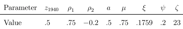
The parameters of the model are presented in table 1
Table 1: Parameter values in the model
Parameter z1940 ρ1 ρ2 a µ ξ ψ ζ
Value .5 .75 −0.2 .5 .75 .1759 .2 23
[image:18.612.110.479.289.508.2]Table 2 presents the identifying moments used to calibrate the model.
Table 2: Identifying moments.
Comparison between the model and the data in 1990
Moment Model Data US, 1990
Skill Premium 1.88 1.878
Skilled workers .87 .949
Consumption Output Ratio .83 .7910
Primary students over Labor Force .177 .16411
Expenditure per pupil over GDP per worker .1258 .113212
Capital Share of GDP .2915 .3
Wage expenditure in education .7036 .703613
σS,U
σS,K 2.62 2.49
14
8Return to 8 years of schooling calculated as exp(ω
t8), where ωt equals the return to one year of high
school for "All men" reported by Goldin and Katz (1999).
9From DeLong, Goldin and Katz (2003) average between 1980 and 2000 for workers with less than 8 years of schooling.
10This is the ratio of Personal Consumption Expenditures to Personal income reported by the Bureau of Economic Analysis, in its table 2.1 for the year 1990
11Calculated as the ratio of students enrolled in primary school times the participation rate over the total labor force. Source: Statistical Abstract of The US for 1994 (data taken for 1990).
12Obtained from the Statistical Abstract of the US 1990 13Obtained from the Statistical Abstract of the US for 1990 14σ
S,U equals the partial elasticity of substitution between S and U. Therefore, σσS,KS,U is the ratio of partial
4.2.2. US Data
In order to construct the series for GDP per worker for the US, I take data from 1950 to 2000
from Heston, Summers and Aten (2002) and add to that data from 1940 to 1950 from the
NIPA tables. I extend the data backwards to capture the 1940s phenomenon that the skill
premium displayed a decreasing trend, contrasting the behavior after 1950. Additionally,
1940 is the first point in time where the data for skill premium is collected from census
sources. From an economic point of view there seems to be evidence that starting in WWII
the availability of technologies may have increased. That is, we can think of the set of
technologies being expanded during the war and from that point on economic agents can
endogenously choose technologies that were not available before15.
The results are not sensitive to the choice of future paths of GDP per worker as long as
abrupt changes close to the data window are not introduced16.
Since this paper focuses on the long run behavior of the economy, the series of GDP per
worker is smoothed using a Hodrick Prescott filter.
Following DeLong, Goldin and Katz (2003), the number of skilled workers in the US,
is taken from decennial census data from 1940 to 2000. A skilled worker is defined as an
individual with educational achievement higher than primary school. The reason for using
a relatively low cutoffis that in poor countries a large fraction of the workforce has less than
6 years of schooling.
The skill premium data for the US, is constructed using the return to High School reported
by Goldin and Katz (1999) from 1940 onwards. The evolution of different measures of skill
premium, such as the return to high school and college indicate an U shape pattern with a
minimum around 1950.
Other data used to calibrate the model come from standard sources.
15In their study Baier et al (2004) find that TFP was constant up to 1940 and in that year it stated increasing in an almost linear way.
Consumption-output ratio, is taken from the NIPA tables and educational expenditures per
pupil over GDP per worker and expenditures in educational wages over total educational
expenditures are obtained from the Statistical Abstract of the US.
5. US Dynamics
The goal of this section is to analyze the endogenously generated dynamics of the skill
premium and skill bias once the economy is confronted with a path of total factor productivity
that perfectly matches the evolution of the GDP per worker in the US after 1940.
For this experiment the US economy is assumed to be in steady state before 194017. At
that point it is assumed that the set of available technologies expanded. This does not imply
that the new technologies would be adopted immediately. The growth in TFP induces the
adoption of those technologies as the stocks of physical and human capital become available.
The idea in the experiment is that these technologies were available from the beginning of
time but were slowly implemented as total factor productivity grew.
The model determines the stock of capital, unskilled workers, skilled workers, their
dis-tribution across the educational and production sectors, their prices and the bias in the
technology. The results in terms of dynamics for the US are shown in the next set of
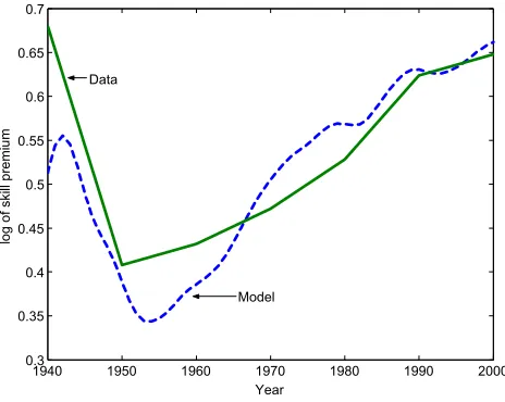
figures18. The endogenous dynamics in terms of skill premium implied by the model are
shown in Figure 5.1. The model provides a unified explanation for the evolution of the skill
premium both before and after 1950. The U shape in the skill premium is generated with
an endogenous skill biased technological change. During the whole period endogenous skill
biased technological change is generated, not only after 1950 as previously explored by the
literature. This effect is generated by the simultaneous effects of technological change and
17Even though the starting point matters for the dynamics of the model, the main results remain valid if the model is started at different points in time, both before and after 1940.
investments in skills and physical capital as depicted in Figure 5.2.
1940 1950 1960 1970 1980 1990 2000 0.3
0.35 0.4 0.45 0.5 0.55 0.6 0.65 0.7
Year
lo
g
o
f
s
k
ill
p
re
m
iu
m
[image:21.612.190.422.134.319.2]Model Data
Figure 5.1: Skill premium in the US from 1940 to 2000 in the data and predicted by the model
The decomposition of the skill premium into the technological factor, the relative supply
of skills factor and the capital deepening factor is shown in Figure 5.2.
From Figure 5.2 it is clear that the decreasing phase of the skill premium up to around
1950 is primarily determined by the behavior of the ratio unskilled to skilled workers devoted
to production. Later, it is the effects of the technological change and investment in physical
capital that determine the increase in skill premium.
The intuition behind the initial reaction is that once the economy is faced with the new
paths for total factor productivity, it starts producing skilled workers at a high rate since
it has to get to a higher level of skilled workers in the new equilibrium and also because
it is experiencing a faster rate of obsolescence of its existing stocks. But after the initial
effects heavily driven by skills creation, investment in physical capital and technological
change become more important and determine an increase in the skill premium. Changes in
technology directly affect the marginal productivities of skilled workers vs. unskilled ones,
but the term based on capital per unskilled worker is affected by both decreasing stocks of
1940 1950 1960 1970 1980 1990 2000 -2.5 -2 -1.5 -1 -0.5 0 0.5 1 1.5 2 L M N "Technology" "Capital Deepening" "Relative Skills"
Figure 5.2: Decomposition of skill premium from 1940 to 2000 ; L = ln³(1−bb)´; M = (ρ2−1) ln³Sp
Up
´
;and N =³1−ρ2
ρ1
´
ln³a+ (1−a)³Kp
Up
´ρ1´
in the skill premium. Even though capital and skills depreciate in the same way as a result
of technological change, since δs < δk, the stock of skilled workers is relatively (to its steady
state evolution) more affected by the accelerated obsolescence induced by the evolution of
bt. Therefore the initial response to TFP favors the creation of skills.
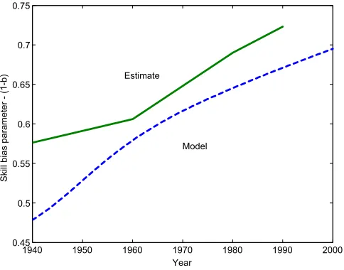
The key element in the model is the skilled biased technological change. In the model
it is endogenous and expressed by the variable (1−bt). The dynamic evolution of that
variable is shown in Figure 5.3. Where we see both the results implied by the model and
the estimates from the data, and in both cases a transition towards a technology intensive
in terms of skill premium is observed. In order to estimate the skill bias parameter shown
in Figure 5.3 I calculatebt as:
bt =
skpt h
a+ (1−a)³Kpt
Upt
´ρ1i ρ2 ρ1 −1 a ³S pt Upt
´ρ2−1 + 1
where skpt represents the skill premium at time t.19
The model delivers endogenous skill bias technological change, which is a direct result
of increases in the exogenous path for TFP. As TFP grows, the economy can devote more
resources to the production of skilled workers and once more skilled workers are available it
is optimal to undertake production under ever more skill intensive technologies.
1940 1950 1960 1970 1980 1990 2000 0.45
0.5 0.55 0.6 0.65 0.7 0.75
Year
S
k
ill
b
ia
s
p
a
ra
m
e
te
r
-
(1
-b
) Estimate
[image:23.612.186.428.230.420.2]Model
Figure 5.3: Evolution of the skill bias parameter(1−b)in the US from 1940 to 2000, predicted by the model and estimated from the data
In other words, once the economy is confronted with a new path for TFP this changes
the demand for skilled workers and physical capital, since the equilibrium technology shifts
towards a new one more intensive in skilled workers. The initial decreasing phase in the
evolution of the skill premium is driven by rapid changes in the ratio of unskilled to skilled
workers devoted to the production sector. Both skilled and unskilled workers are reallocated
as a result of the new path of total factor productivity to the educational sector in greater
numbers than in the previous steady state. This reallocation is driven by two forces. First,
when total factor productivity is higher, so is the steady state level of(1−b)and, therefore,
19Using the data forS
pt andUpt, Kt and the skill premium and the parameters chosen in the calibration
1940 1950 1960 1970 1980 1990 2000 0.4
0.6 0.8 1
Skilled Workers
1940 1950 1960 1970 1980 1990 2000 0.2
0.25 0.3 0.35 0.4
Capital Share of GDP Data
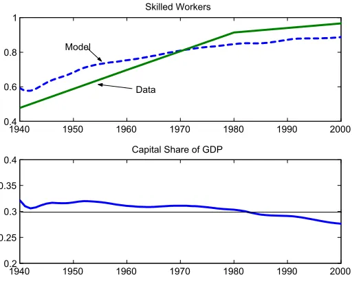
[image:24.612.178.434.106.314.2]Model
Figure 5.4: Evolution of the stock of skilled workers over labor force and the capital share of GDP
the optimal level of skilled workers is also higher, given that their marginal product grew.
Second, during the transition the rate at which the stocks of skilled workers become obsolete
is higher than in the steady state equilibrium. Therefore, in equilibrium the economy chooses
a higher level of skilled workers and higher rate of obsolescence, which implies that more and
more resources are devoted to the educational sector at the expense of the production one.
The increasing phase in skill premium post 1950 is generated almost exclusively by the
changes in technology and the increases in physical capital into the production sector that
enter in full effect after the stocks of skilled workers had been created and can enter the
production sector.
As independent evaluation of the model, the evolution of the capital share of GDP and
the evolution of the stock of skilled workers are reported in Figure 5.4. Capital share, over
the period 1940 - 2000, remains close to30%, which is what many studies suggest should be
the number for the US20. In terms of the ratio of skilled workers to total labor force, the
model predicts a range smaller than what the data suggests, but still it captures most of its
evolution.
6. Cross Country Evidence
This section serves a dual purpose. First it serves as an independent evaluation of the
model, because the same parameter values that were obtained from the calibration for the
US are used in the cross country context. Second, it endogenously generates the evolution of
the skill premium and technology adoption for different countries, with completely different
paths for GDP per worker, matching its cross section around 1990.
In order to conduct cross-country comparisons, an international database is set up.
In-stead of following individual countries I follow deciles of the GDP per worker distribution
in 199021. GDP per worker is computed as an unweighted average per decile for the
coun-tries with long enough series (those with complete series from 1960 to 1996), from Heston,
Summers and Aten (2002), expanded back to 1940 taking the average growth rate in the
period (1960-1965). The stock of skilled workers is computed using data from Barro and Lee
(1993), using the same definition as for the US case. The skill premium is computed using
data from returns to schooling from Bils and Klenow (2000), and the duration of primary
school as Caselli and Coleman (2006).
6.1. Experiment
The experiment across countries is the following: Begin in 1940 in steady state for every
decile of the distribution of the GDP per worker and choose a sequence of TFP that matches
the evolution of GDP per worker for each decile from 1940 to 2000, and impose convergence
to a decile specific level by taking the last 5 years of data and letting the growth rate of
GDP per worker decrease linearly from the average growth rate from the last 5 years to 0 in
50 years, and after that stay constant for ever.
0 0.1 0.2 0.3 0.4 0.5 0.6 0.7 0.8 0.9 1 0.8
0.85 0.9 0.95 1 1.05 1.1 1.15 1.2 1.25
GDP per worker relative to US
S
k
ill
P
re
m
iu
m
r
e
la
ti
v
e
t
o
U
S
Model
[image:26.612.189.422.131.316.2]Data
Figure 6.1: Skill premium as a fraction of the US in the data and model across deciles of the world distribution of GDP per worker
With this strategy it is possible to compute a dynamic path for every 1990-decile. When
comparing the data to the model, I take the 1990 cross section and, therefore, I take the
transitional point that corresponds to 1990 in the model. I compute the skill premium
as exp((ωn)i) where ωn is the median by decile of the skill premium and ω represents the
coefficients for schooling in the Mincer regressions reported by Bils and Klenow (2000)22
and n the length of the primary school in years from Caselli and Coleman (2006)23. The
comparison between the model and the data is reported by Figure 6.1
The model is shifted to the right with respect to the data, but it is in the right scale
and predicts a hump shape in skill premium, much as the one obtained from the data. As
in the US case, the skill premium can be decomposed into three terms which depend on
22An additional complication arises with the comparison between model and data in terms of skill premium across deciles, because we do not have data gathered in the same year across countries, so instead of checking what the model implies for 1990 in terms of skill premium, I take the average by decile of the year in which the observation reported by Bils and Klenow (2000) was made and bring that number from the model for each decile.
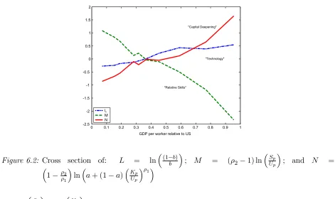
0 0.1 0.2 0.3 0.4 0.5 0.6 0.7 0.8 0.9 1 -2.5 -2 -1.5 -1 -0.5 0 0.5 1 1.5 2
[image:27.612.70.541.99.379.2]GDP per worker relative to US L M N "Technology" "Relative Skills" "Capital Deepening"
Figure 6.2: Cross section of: L = ln³(1−bb)´; M = (ρ2−1) ln³Sp
Up
´
; and N = ³
1−ρ2
ρ1
´
ln³a+ (1−a)³Kp
Up
´ρ1´
¡1−b b
¢ ,³Sp
Up ´
and³Kp
Up ´
. Figure 6.2 depicts the influence of each term in the skill premium
pattern across countries around 1990.
Even though the model predicts that countries will adopt ever more skill biased
technolo-gies as they develop, the dominating mechanisms in terms of the cross-country comparison
of the skill premium are those generated by differences in the capital to unskilled worker
ratio and the skilled to unskilled workers ratio in the production sector
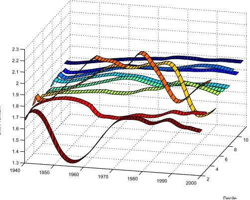
Even more interesting is the dynamic behavior for skill premium for all the deciles over
time. The fact that they follow different trajectories of TFP so as to match GDP per worker
makes the skill premium differ greatly in terms of its dynamic path across deciles. Figure
6.3 depicts the whole path for each decile from 1940 to 2000, where the U shape pattern
displayed by the US and thefirst decile (induced by the US) is not generic to any departure
from steady state. Both the initial conditions and future path of TFP matter in terms of
reaction for the economy in terms of skill premium.
What is clear from Figure 6.3 is that the reaction of the skill premium differs from decile
10 8 6 4 2 1940 1950
1960 1970
1980 1990 2000 1.3
1.4 1.5 1.6 1.7 1.8 1.9 2 2.1 2.2 2.3
Decile
S
k
ill
P
re
m
iu
[image:28.612.175.426.119.320.2]m
Figure 6.3: Skill premium predicted by the model across deciles from 1940 to 2000
Deciles 3 and 4 start in 1940 with increases in skill premium but then decline by 1980. In
the remaining deciles there seems to be a small change in skill premium. The differences
across deciles arise from differences in the initial conditions and the paths of total factor
productivity necessary to match the evolution of GDP per worker.
In terms of technology adoption, the parameter (1−b) chosen across deciles is depicted
in Figure 6.4. There it is clear that the production technology in use in the higher deciles
is relatively more intensive in the use of skills. Also, those countries with GDP per worker
above half the level of the US are very close in terms of skill bias technology, whereas the
poorer half of the distribution chooses a fairly different technology
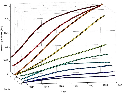
Figure 6.5 presents the dynamic behavior across deciles of the parameter(1−b)from 1940
to 2000. There, it is the top 4 deciles which have incurred major technological change, and
the rest of the distribution remained with a technology that did not change much over this
period, suggesting the existence of "technology adoption clubs", where the richer countries
adopt more skill intensive technologies faster than the poor ones generating a pattern of
0 0.1 0.2 0.3 0.4 0.5 0.6 0.7 0.8 0.9 1 0.4
0.45 0.5 0.55 0.6 0.65
GDP per worker relative to US
S
k
ill
b
ia
s
p
a
ra
m
e
te
r
(1
-b
[image:29.612.195.417.102.282.2])
Figure 6.4: Skill bias parameter(1−b) across deciles in 1990
parameter(1−b)has diverged across deciles, from a range from .4 to .48 in 1940 to between
.43 to .65 in 2000.
I find that richer countries endogenously choose technologies that are intensive in the use
of the skilled labor factor, but the adoption of these technologies is far from linear in the
level of development. The results show the existence of technology adoption clubs at the
top half of the distribution of GDP per worker.
As an independent evaluation of the model, Figure 6.6, shows the evolution of the stock
of skilled workers across deciles in 1990. The model’s overprediction the stock of skilled
workers is a direct consequence of the fact that it is calibrated to US, data which can be
considered an outlier even in the top decile. Therefore , apart from the scale bias discussed
above, the model predicts the correct relationship between the stock of skilled workers and
level of GDP.
7. Conclusion
The literature on skill biased technological change argues that it explains the observed
2 4
6 8
10
1940 1950 1960 1970 1980 1990 2000 0.45
0.5 0.55 0.6 0.65
Year Decile
s
k
ill
b
ia
s
p
a
ra
m
e
te
r
(1
-b
[image:30.612.185.419.116.295.2])
Figure 6.5: Skill bias parameter (1−b) across deciles from 1940 to 2000
technology adoption decision, and generate endogenous skill biased technological change that
is consistent with the data for the US time series and the cross country evidence in terms of
skills formation and skill premium.
The model has potential in explaining why it is that poor countries do not adopt newer
technologies when they are readily available and implemented in more advanced countries.
The fact that there is a cost associated with changing the technology in terms of inputs makes
that transition costly and may take long periods of time. It is an alternative argument to
the barriers of adoption argued by Parente and Prescott (2000). Here, instead of monopoly
groups protecting their rents, it is optimal in a competitive setting to delay the adoption of
more advanced technologies in the face of technology adoption costs.
Total factor productivity still plays a major role in the paper suggesting that there may
still be a channel similar to that of Parente and Prescott (2000), in the sense that T.F.P.
0 0.2 0.4 0.6 0.8 1 0.2
0.3 0.4 0.5 0.6 0.7 0.8 0.9 1
GDP per worker relative to US
F
ra
c
ti
o
n
o
f
s
k
ill
e
d
w
o
rk
e
rs
Model
[image:31.612.189.418.103.291.2]Data
Figure 6.6: Skilled workers across deciles in 1990
References
[1] Acemoglu, Daron. 2002. Directed Technical Change. The Review of Economic Studies,
69: 781-809.
[2] Baier, Scott, Sean Mulholland, Robert Tamura and Chad Turner. 2004. How Important
are Human Capital, Physical Capital and Total Factor Productivity for Determining
Economic Growth in the United States, 1840 - 2000, Clemson University mimeo.
[3] Barro, Robert J. and Jong-Wha Lee. 1993. International Comparisons of Educational
Attainment. Journal of Monetary Economics, 32(3): 363-394.
[4] Bils, Mark, and Peter Klenow. 2000. Does Schooling Cause Growth?. American
Eco-nomic Review, 90(5):1160:1183.
[5] Caselli, Francesco and Wilbur John Coleman II. 2006. The world Technology frontier.
American Economic Review, 96(3): 499-522.
[6] Chari, V.V. and Hugo Hopenhayn. 1991. Vintage human capital, growth and the
[7] DeLong, J Bradford, Claudia Goldin and Lawrence Katz. 2003. "Sustaining US
Eco-nomic Growth". In Agenda for the Nation, H. Aaron, et al., eds., 17-60, Washington,
D.C.: The Brookings Institution.
[8] Funk, Peter and Thorsten Vogel. 2004. Endogenous skill bias. Journal of Economic
Dynamics & Control, 28: 2155-2193.
[9] Goldin, Claudia and Lawrence Katz. 1999. "Decreasing (and then increasing)
Inequal-ity in America: A Tale of Two Half-Centuries". In The Causes and Consequences of
Increasing Income Inequality, F. Welch, ed., 37-82, Chicago: University of Chicago
Press.
[10] Greenwood, Jeremy and Mehmet Yorokoglu. 1997. 1974.Carnegie-Rochester series on
public policy, 46(6): 49-95.
[11] Hamermesh, Daniel. 1993. Labor Demand. Princeton: Princeton University Press.
[12] Heckman, James, Lance Lochner and Christopher Taber. 1998. Explaining rising wage
inequality: Explorations with a dynamic general equilibrium model of labor earnings
with heterogeneous agents. Review of Economic Dynamics, 1: 1-58.
[13] Heston, Alan, Robert Summers and Bettina Aten. 2002. Penn World Table Version 6.1,
Center for International Comparisons at the University of Pennsylvania (CICUP).
[14] Hubbard, Glenn, Jonathan Skinner and Stephen Zeldes. 1994. The importance of
pre-cautionary motives in explaining individual and aggregate saving. Carnegie-Rochester
Conference Series on Public Policy, 40: 59-125.
[15] Jovanovic, Boyan. 1998. Vintage capital and inequality.Review of Economic Dynamics
1: 497-530.
[16] Jovanovic, Boyan and Yaw Nyarko. 1996. Learning by doing and the choice of
[17] Krusell, Per, Lee Ohanian, Jose Rios-Rull and Giovanni Violante. 2000.
Capital-Skill Complementarity and Inequality: a macroeconomic analysis.
Econometrica, 68(5): 1029-1053.
[18] Manuelli, Rodolfo and Ananth Seshadri. 2004. Human Capital and the Wealth of
Nations. University of Wisconsin - Madison, Mimeo.
[19] Murphy, Kevin, Craig Riddell and Paul Romer. 1998. Wages, Skills and Technology
in the United States and Canada. NBER Working Paper 6638.
[20] Parente, Stephen and Edward Prescott. 2000. Barriers to Riches. Cambridge: MIT
Press.
[21] Uzawa, Hirofumi. 1962. Production Functions with constant elasticities of substitution.
8. Appendix 4: Data
8.1. US data
The data for the dynamic analysis concerning the US was constructed as follows:
GDP per worker: The figures for GDP per worker comes from Heston, Summers and
Aten (2002) for the period 1950 - 2000. For the periods 1940-1950 and 2001-2004 the series
is complemented with data from the BEA constructed as GDP/Labor force. The series is
smoothed with a Hodrick Prescottfilter with parameter equal to 100, since these are yearly
data. Finally I make the series converge to a future steady state by taking the average
growth rate for the period 1999 - 2004 and make it decline linearly for 50 years to zero.
After that GDP per worker stays constant into the infinite future.
Skilled workers: The definition of skilled workers is "those with more than primary
schooling". Obtained from DeLong, Goldin and Katz 2003, Figure 2.4.
Skill Premium: The skill premium data is constructed from Goldin and Katz (1999).
They report returns to High School and College for young men and all men. I take the
return to High school for all men as the return to education for each year. The return to
8 years of schooling calculated as exp(ωt8), where ωt equals the return to high school "All
men" reported by Goldin and Katz (1999).
Skill bias parameter b: In order to construct the skill bias parameter shown in Figure
5.3 I calculated the skill premium as skpt= wst wut =
(1−bt)
bt
Sρ2−1 pt
[aUρ1
pt+(1−a)K ρ1 pt]
ρ2
ρ1−1aUρ1−1 pt
Therefore we can recover the parameter bt asbt= skpAt+tAt
where At=
Sρ2−1 pt
[aUρ1
pt+(1−a)K ρ1 pt]
ρ2
ρ1−1aUρ1−1 pt
Using the data described above and the parameters chosen in the calibration shown in
table 1, I was able to construct a series for At. The only missing data was the evolution
of Kt. And, not only that, but also the fact that there is a scale issue with the capital
Fixed reproducible Tangible Wealth series as do Baier et al (2004). In order to solve the
scale issue I use the model to guide my decision. In the model K1940 = 0.7043, therefore I
rescaled the whole series of capital stocks such that it matches the model in 1940.
Consumption Output ratio in 1990: Obtained as the ratio of personal consumption
expenditure to personal income reported by the BEA in table 2.1.
Primary students over labor force in 1990: Obtained from the Statistical Abstract for
the US for 1994 (checking the 1990 data). Is the ratio of enrolled primary students *
participation rate over labor force.
Expenditure per pupil over GDP per worker in 1990: Taken as the ratio of expenditures
in primary schooling over enrolled students and that ratio divided by GDP per worker.
Source Statistical Abstract of the US 1994, for year 1990.
Wage expenditure in education in 1990: Taken from the Statistical Abstract for the US
1994 for year 1990. Is the ratio of wage expenditures to total expenditures in education.
Ratio of elasticities of substitution: Taken from Hamermesh (1993), and Krusell et al
(2000).
8.2. Cross Country data
Countries: The countries included in the database are those which fulfill the following
crite-ria: Have skill premium data, have long enough GDP per worker data, have data on skilled
workers as specified in the next set of items.
Table 3: Countries included in the cross country database24
Argentina El Salvador Kenya Sri Lanka
Australia France Korea, Rep. of Sweden
Bolivia Ghana Malaysia Switzerland
Botswana Greece Mexico Taiwan
Brazil Guatemala Netherlands Thailand
Canada Honduras Nicaragua Tunisia
Chile Hong Kong Pakistan United Kingdom
China India Panama United States
Colombia Indonesia Paraguay Uruguay
Costa Rica Israel Peru Venezuela
Cyprus Italy Philippines
Dominican Rep. Jamaica Portugal
Ecuador Japan Singapore
With that list of countries, I ordered them by GDP per worker in 1990 and constructed
deciles. Then I followed the 10fictional countries constructed as averages of GDP per worker
per decile over the period 1940 - 2240.
GDP per worker: The list of countries above includes the countries with long enough
data for GDP per worker in Heston, Summers and Aten (2002) for the period 1960 -1996. If
a country does not have a complete series of GDP per worker for the mentioned period it was
deleted from the database. The GDP per worker for the years 1940 to 1960 was constructed
as a constant growth rate equal to that in the first 5 years of data, and the convergence
to a final steady state was created following the same procedure as for the US. Then I
averaged GDP per worker over deciles and made the series of GDP per worker converge to
a decile specific steady state following the procedure used for the US data. The data was
also smoothed with a Hodrick Prescottfilter with parameter equal to 100.
Skill premium: Using the returns from Bils and Klenow (2000) and the duration of
primary school used by Caselli and Coleman (2006) I construct the skill premium exp((ωn)i)
where ωn is the median by decile of the skill premium and ω represents the coefficients for
schooling in the Mincer regressions reported by Bils and Klenow (2000) andn the length of
the primary school in years from Caselli and Coleman (2006). An additional complication
arises with the comparison between model and data in terms of skill premium across deciles,
because we do not have data gathered in the same year across countries, so instead of
checking what the model implies for 1990 in terms of skill premium, I take the average by
decile of the year in which the observation reported by Bils and Klenow (2000) was made
and bring that number from the model for each decile. The result is reported by Figure
6.1. The countries that are in the Bils and Klenow (2000) database and are dropped here
are: Germany, Hungary and Poland. These countries were dropped because the GDP per
worker series was not long enough (from 1960 to 1996).
Skilled workers: The stocks of skilled workers, defined as "those with more than primary