Munich Personal RePEc Archive
U.S. Core Inflation: A Wavelet Analysis
Cotter, John and Dowd, Kevin
University College Dublin
2006
U.S. Core Inflation: A Wavelet Analysis
by
Kevin Dowd*
Nottingham University Business School
Phone: +44 115 846 6682; Fax: +44 115 846 6667
Email: [email protected].
and
John Cotter
University College Dublin,
Phone +353 1 7168900
Email: [email protected].
Revised, September 10, 2006
* Kevin Dowd is Professor of Financial Risk Management at Nottingham University Business School.
2
Running Head: U. S. Core Inflation
Name and mailing address of corresponding author:
Kevin Dowd
Nottingham University Business School,
Jubilee Campus,
Wollaton Rd,
Nottingham NG8 1BB,
3 Abstract
This paper proposes the use of wavelet methods to estimate U.S. core inflation. It
explains wavelet methods and suggests they are ideally suited to this task.
Comparisons are made with traditional CPI-based and regression-based measures for
their performance in following trend inflation and predicting future inflation. Results
suggest that wavelet-based measures perform better, and sometimes much better,
than the traditional approaches. These results suggest that wavelet methods are a
promising avenue for future research on core inflation.
4
1. INTRODUCTION
Monetary economists have long understood that some measures of inflation are more
important, or more revealing, than others, and the distinction between headline
inflation and underlying, or core, inflation, has been recognised for many years.
However, interest in core inflation took off only in the 1990s.1 As inflation targeting
became more widespread, central bankers became more concerned to find the ‘right’
inflation rate to target, or to use as a monetary policy indicator; and as inflation fell,
disentangling inflation signals from inflation noise became more critical to successful
monetary policy decision-making: to paraphrase Blinder (1997, p. 158), when
inflation is high, the central bank knows it has to lower inflation, regardless of how it
is measured; but when inflation is low, different measures of inflation can suggest
different monetary policy decisions, and correctly extracting the inflation signals
becomes critical.
The literature on core inflation suggests two alternative definitions of the
term. Some authors define core inflation as an inflation measure that represents
underlying or trend inflation (e.g., Bryan et al., 1997, Cecchetti, 1997), whilst others
1 The term ‘core inflation’ goes back at least to Eckstein (1981, p. 7), who defined it as the “trend
5
define core inflation as a leading indicator of future inflation (e.g., Blinder, 1997,
Smith, 2004). In practice, we would often like a core inflation measure that is
compatible with both definitions – namely, is a good representation of underlying
trend inflation and is a good indicator of future inflation. Thus we analyse two
performance criteria (and separate associated test methodologies) to determine
whether the candidate core inflation measures are able to match the alternative
definitions of core inflation (i.e., in terms of tracking a trend and predicting future
inflation).2
We can also think of core inflation as follows. We start with a given
original or ‘parent’ inflation series, whose ‘core’ it is that we are seeking. We can
then regard core inflation as some series that is closely related to the ‘parent’ series,
but that also satisfies certain desirable properties such as capturing the trend,
predicting the ‘parent’ series, and so forth.
Much of the literature on core inflation in the U.S. has taken the ‘parent’
inflation rate to be the CPI and examined measures of core inflation derived directly
longstanding debate on inflation measurement that goes back to Irving Fisher and earlier. For more on these issues and the origin of the notion of core inflation, see, e.g., Wynne (1997) and Roger (1998). 2 Ideally, we might also want a measure of core inflation to satisfy a number of additional criteria (see
6
from the components that make up the aggregate CPI index.3 The most widely used
such measure is ‘CPI less food and energy’ – inflation measured on the basis of a
reconstructed CPI that gives food and energy components a zero weight. There are
also related measures – inflations based on ‘CPI less energy’, ‘CPI less food’, the
median CPI, and various ‘trimmed mean’ CPIs. The use of ‘CPI less x’ measures of
core inflation is sometimes justified on the grounds that the excluded terms
(supposedly) have more noise than the included terms, and the median and trimmed
mean measures can be justified on robust statistics and other grounds (see, e.g.,
Bryan et alia, 1997). Core inflation measures are also sometimes obtained using
regression-based methods, which can be regarded as producing optimal measures of
core inflation given assumptions about the trend itself and the noise around it. These
methods include moving averages, exponential (and other) smoothing methods and
time series (Box-Jenkins) methods.
This paper proposes some new core inflation measures based on a recently
developed approach – wavelet analysis – that is ideally suited to the estimation of
core inflation. The motivation for these measures is the simple idea that if core
inflation is to be interpreted as an underlying signal from an original noisy inflation
process, then we should be able to estimate core inflation using a suitable signal
extraction or denoising method, but we need a method that takes account of the
non-stationarity (and general ‘bad behavedness’) of real-world inflation series. Wavelet
7
methods are specifically designed for this type of problem and have been used with
great success in many areas of applied science and engineering. Wavelet methods
avoid the arbitrariness of those approaches that estimate core inflation simply by
excluding certain components from the ‘parent’ inflation rate. But unlike
conventional statistical methods of detrending data, wavelet methods do not require
strong assumptions about the trend or the noise around it. Indeed, a particular
strength of wavelet methods is that they have no problems dealing with time-varying
behavior that incorporates non-stationarity, jumps or discontinuities, regime shifts,
isolated shocks, and similar times-series behavior, such as we see in many inflation
rate series. Wavelet methods are therefore ideal for signal extraction problems such
as the measurement of core inflation. 4
This paper is laid out as follows. Section 2 briefly reviews some of the
existing literature on core inflation in the United States. Section 3 introduces wavelet
methods. Section 4 explains their suitability for estimating core inflation and shows
how they can be applied to this purpose. Section 5 explains the data, and section 6
presents our results. Section 7 concludes.
et al. (1997), Cecchetti (1997), Clark (2001), Cogley (2002), Smith (2004), and Wynne (1997). 4 As well as the two performance criteria applied of trend tracking and predictability it is clearly
important to be able to apply wavelet analysis in real-time contexts. Here we would want the wavelet measures of core inflation to update the estimates based on the arrival of new data in a reliable fashion. This is a developing area, and applications have been made on real-time problems such as processing new ethernet and ATM data using Abry-Veitch wavelet-based estimators (see Roughan et alia, 2000).
8
2. EXISTING MEASURES OF CORE INFLATION
2.1. CPI-based measures of core inflation
Many common measures of U. S. core inflation are derived from the CPI as the
‘parent’ inflation series. Perhaps the most widely used such measure is ‘CPI inflation
less food and energy’ – the CPI inflation rate constructed with zero weights attached
to the food and energy components – which has long been used as a measure of core
inflation in the U.S. This measure is often motivated informally on the grounds –
valid or otherwise – that food and energy are subject to a lot of high frequency
variation (e.g., due to weather, seasonality, etc) that injects noise into CPI inflation
signals. It is argued that cutting out these components eliminates this noise and so
gives a better indicator of underlying (i.e., core) inflation. We can also cut out these
components individually to give us two different core inflation measures – ‘CPI less
energy’ and ‘CPI less food’ – that can be motivated on similar grounds, and we can
cut out other components as well. These measures have the advantages that they are
easily understood, timely and not subject to revision. However, the choice of
excluded components is arbitrary, such measures fail to address relative price shocks
9
within included components, and the excluded components may not be more volatile
than included ones.5
A common alternative is the median CPI inflation rate, proposed by Bryan
and Cecchetti (1994), Bryan et al. (1997), Apel and Jansson (1999), and others. The
median has the advantage that it does not require the arbitrary selection or deselection
of components in advance. It is also more robust than the CPI inflation rate to large
shocks in individual components; its use can therefore be justified by reference to the
theory of robust statistics (i.e., that in the presence of skewness and other
non-normality, the median is a more efficient estimator of the population mean than the
sample mean). Its use can also be justified by the economic argument that in the
presence of menu costs, firms will only change prices in the face of large shocks; in
such circumstances, the median would be a better estimate of the underlying inflation
than the mean. However, the median excludes components experiencing relatively
large price changes and when used as a measure of core inflation may therefore miss
price changes that provide useful information on trend inflation (Cockerell, 1999;
Clark, 2001). It has also been said that central banks may not wish to use the median
as a measure of core inflation on the grounds that the median is not well nderstood by
the public (Rogers, 1998; and Álvarez and Llanos, 1999).
5 Most empirical studies seem to suggest that CPI less food and energy is a poor measure of core
10
Closely related are the trimmed mean measures.6 These are the means of
the ordered, weighted component inflation rates, with the upper and lower tails
excluded. For example, the 9% trimmed mean is the mean constructed from the
ordered weighted component inflation rates, with the bottom 9% and top 9% of
changes excluded. The use of these measures can also be justified by robust statistics
theory and/or economic menu-cost arguments, and they too do not require arbitrary
decisions on what components should be included or excluded.7 However, trimmed
measures arguably suffer from similar problems as the median.
2.2. Regression-based measures of core inflation
Regression methods provide a rather different approach to core inflation
measurement. If we define core inflation in terms of a trend, then the estimation of
core inflation requires estimation of a trend and – provided we feel comfortable with
the statistical assumptions involved – regression methods provide a straightforward
way to estimate this trend: we specify our underlying assumptions about the trend
6
There are also other related measures. For example, there are the volatility-weighted (or Edgeworthian) measures, proposed by Dow (1994), Diewert (1995), Wynne (1997, 2001) and Vega and Wynne (2001). These are based on the idea that we should weight price changes by volatility, so giving more volatile components a lower weight and getting a more accurate aggregate price signal. Since volatility erodes the relative price signal, we volatility-adjust the weights to get a more reliable aggregate signal. These have the advantage over median and trimmed mean estimators of not throwing information away, but constructing weights can be difficult and the weights themselves can be unreliable.
7 Most studies seem to agree that these median and trimmed means measures generally perform better
11
itself (e.g., whether it is linear, quadratic, etc.); we specify the nature of the the
departures from it, which can be regarded as the equation’s errors (e.g., these might
be normal, autocorrelated, etc.); and we apply the appropriate regression method.
These methods include simple moving averages of current and past inflation, time
series methods such as Box-Jenkins ARMA and ARIMA methods,8 and statistical
smoothing methods, such as the exponentially smoothed core inflation estimator
recently proposed by Cogley (2002).9 Regression-based methods avoid the
arbitrariness of including or excluding particular components, are easy to use, and
can be applied in real time if we estimate regressions on a rolling basis. They also
have the attraction that a suitable choice of regression method can provide us with an
optimal trend – and hence an ‘optimal’ core inflation measure – given the
assumptions we make. However, their disadvantage is that we have no easy way to
verify what these assumptions should actually be. In practice, we can rule out the
more obviously naïve assumptions (e.g. that core inflation is constant?) on a priori
grounds or on the basis of suitable tests, but distinguishing between more plausible
alternatives is difficult. In using such methods, we therefore end up having to make
8 There is relatively little clear evidence in the literature on the performance of these measures,
because these measures are usually used in this area to provide proxies for trend inflation against which other measures of core inflation can be assessed. In this paper, by contrast, we are concerned
with these estimators as measures of core inflation in their own right.
9 This estimator has a number of attractive features as a measure of core inflation (e.g., it depends on a
12
certain assumptions on faith, and the value of our results may be dependent on the
validity of these untested assumptions.
3. WAVELET METHODS
A wavelet can be defined as a “waveform of effectively limited duration that has an
average value of zero” (Misiti et al. (2000, p. 1-9)). More informally, we can think of
a wavelet as a localised waveform in time-scale space. Wavelet analysis consists of
taking a chosen waveform, the so-called mother wavelet, and breaking up a signal or
series into shifted (i.e., in time) and scaled (i.e., compressed and extended) versions
of the mother wavelet. Unlike classical wave (i.e., Fourier) analysis,10 a wavelet does
not require strong statistical assumptions and can be applied to ‘difficult’ signal
processing problems such as the detection of underlying patterns or trends in
non-stationary series, the removal of noise, and the identification of breakdown points and
discontinuities. Wavelet analysis is a relatively recent development – most of the
seminal work was done in the 1980s – but has proven to be immensely useful in
many diverse areas such as medicine, biology, oceanography, earth studies, and
10 Fourier analysis is limited because it presupposes a stationary signal. The traditional solution to the
13
fingerprint analysis. Wavelets have also been used in a variety of economic and
finance applications, such as the modelling of non-stationary processes (Ramsey and
Zhang, 1997) and long-memory processes (Jensen, 1999), time-series decomposition
(Ramsey and Lampart, 1998), forecasting (Stevenson, 2001), scaling analysis
(Gençay et al., 2002), and outlier testing (Greenblatt, 1994).11
Wavelet analysis is particularly promising for the estimation of core
inflation for several reasons. First and most obviously, wavelet analysis is
tailor-made for the denoising of (or signal extraction from) non-stationary time series, and
these characteristics are ideal for core inflation analysis: the process of obtaining a
core inflation rate is essentially a form of signal extraction, and inflation series are
typically non-stationary. Hence, wavelet analysis has the advantages that it avoids
strong statistical assumptions (unlike, say, regression-based estimates of core
inflation) and has no problems handling the non-stationary behavior of inflation
arising from shifts in monetary policy, oil price shocks, and the like.
Secondly, because wavelet analysis can lead to core inflation series that
have fundamentally different ‘shapes’ over time, we can use it to select a core
inflation series that reflects the reasons why we might want a measure of core
inflation in the first place, i.e., we can choose a core inflation series whose ‘shape’
helps us with the problem at hand. Some wavelet specifications give rise to core
inflation series whose times-series plots are ‘smooth’, whilst others give rise to plots
11 For more on these and other economic applications, see also Gençay
14
that are ‘pointed’ or exhibit ‘plateaux’. Each of these shapes can satisfy a particular
purpose. For example, if we want a core inflation measure that reflects an underlying
trend, we would presumably want our core inflation curve to be smooth. However,
there may be circumstances where we prefer one of the other shapes. For instance, if
we were more interested in capturing the key inflation turning points, we might
prefer a ‘pointed’ shape because this shape highlights the turning points in which we
are primarily interested. Alternatively, we might be interested in distinguishing
between shifts in core inflation, and in this case the ‘plateaued’ [sic] shaped would be
more helpful: each flat plateau represents a particular period of ‘stable’ core inflation,
and shifts from one plateau to another represent a jump from one core inflation rate
‘sub-regime’ to another. Thus, wavelets can be used to produce core inflation
measures that are tailor-made to the context in which we want to use them.12, 13
(2002).
12 Wavelet methods also have another, albeit mixed, blessing. From a filtering point of view, wavelet
analysis can be regarded as a highly efficient form of two-sided filtering with time-varying coefficients, and have the standard advantages of two-sided over one-sided filtering. (For more on these, see, e.g., Gençay et alia, 2002.) So, for instance, in estimating unobservable variables such as
core inflation over a specific time period, wavelet methods can incorporate data from both before and after that time period, and so produce estimates that are superior (from a filtering perspective) than those that can be obtained using only one-sided filters (in which estimates of the current period’s core inflation make use of data available in this period and do not make use of later data that becomes available). This is an advantage in contexts where we might be interested in measuring historical core inflation rates. Nontheless, it is a (potential) disadvantage when operating in situations where we wish to estimate core inflation using only past data for each period concerned, i.e., in many real-time contexts. However, as we have seen in note 4 above, this is not an insurmountable barrier by any means.
13 One potential problem with wavelets applied to core inflation is that they are essentially ‘black box’
15
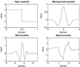
To apply wavelets, we first select a particular wavelet type, and there are
many types to choose from; these have different properties and are useful for
different applications.14 The simplest (and also first known) wavelet is the Haar
wavelet, which is a straightforward step function. A second is the Mexican hat
wavelet with its distinctive ‘Mexican hat’ shape. Other popular wavelets are the
family of Daubechies wavelets. These are distinguished from each other by their
order number – Daubechies 1, Daubechies 2, and so on – and include the Haar
wavelet as a special case when the order is 1. Similar to these are the symlets –
symlet 1, symlet 2, etc. – which are nearly symmetrical relatives of the Daubechies
family.
Some of these wavelet shapes are illustrated in Figure 1. This Figure shows
the discontinuous Haar or step-function wavelet, the unmistakeable Mexican hat
wavelet, a Daubechies 4 wavelet showing the asymmetry of this wavelet family, and
a near-symmetrical Symlet 2 wavelet.
Insert Figure 1 here
‘explained’ to the public: for example, a central bank might use wavelet methods to provide inflation indicators for its own internal analysis. One might also argue that the public has little real understanding of index-number issues in the first place.
14 There exists a considerable technical literature on the different wavelets and their properties.
16
Having selected our wavelet type, we then apply a suitable algorithm. In
most practical cases this would be Mallat’s discrete wavelet transform, which is a
fast and efficient way to estimate the wavelet coefficients (Mallat, 1989). Applying
such an algorithm decomposes our original series into two series – an
‘approximation’ series, which highlights the high-scale, low-frequency components
(or underlying pattern or trend) of the original series, and a ‘details’ series, which
highlights the low-scale, high-frequency components (or noise) of the original series.
If we wish, we can then take the approximation series and filter it again: this gives us
a level 2 approximation. We can repeat the process as often as we wish: filtering the
level 2 approximation gives us a level 3 approximation, and so on. Each time we
apply the filter (or increase the approximation level) we remove more of whatever
high-frequency, low-scale components still exist in our approximation series, and so
obtain a ‘cleaner’ high-scale, low-frequency underlying pattern or trend. We can
therefore think of the application of wavelets as involving both a choice of wavelet
form and a choice of approximation level: decomposing the series once is a level-1
analysis, decomposing twice is a level-2 analysis, and so on.
If we apply this method to a given inflation series, then the suitably
‘cleaned’ approximation series gives us our core inflation, and the original, given,
inflation series is our ‘parent’ inflation. Put another way, we take our ‘parent’ series,
and put it through a wavelet analysis to obtain our core inflation series, and the
choice of wavelet type and approximation level determine how the core inflation
17
4. USING WAVELETS TO ESTIMATE CORE INFLATION15
As we have already mentioned, wavelet analysis involves the application of
successive approximations to remove more and more high frequency detail, or noise,
and so help reveal an underlying signal (or shape). However, if we apply too many
approximations, we also remove parts of the signal itself. A balance therefore has to
be struck so that we don’t lose the signal along with the noise. This means that we
need some guidelines to help draw a reasonable balance, and in this paper we make
use of two particular sets of guidelines:
• Normality of ‘details’: There is a heuristic argument that we should stop
approximating before the details have become normal. More precisely, if the
details at level i are normal, then the ith level approximation merely removed
‘random’ noise, and this would indicate that the ith level approximation was
unnecessary: i.e., no more than i-1 levels are needed.
• Minimum (or, more generally, low) entropy: Applying information theory, the
optimal number of levels is the one with the lowest entropy. More generally,
any reasonable choice for the number of levels should have a relatively low
entropy.
15
18
These considerations suggest the following approach to the selection of
plausible wavelet-based measures of core inflation:
• We start with a reasonable universe of plausible wavelet types,16 where the
initial choice of plausible wavelets might be guided by the context we are
working in: so, for example, if we are seeking a ‘smooth’ core inflation series,
we might restrict ourselves to wavelets that generate a smooth core inflation
series, etc. For each type of wavelet, we consider a reasonable number of
approximation levels.17
• For each wavelet type and approximation level considered, we estimate the
Jarque-Bera (JB) probability values for the details estimated at that level of
approximation, and we note those levels (if any) with reasonable prob-values
(e.g., higher than 1%). If we cannot find any levels with reasonable JB
prob-values, then we eliminate that wavelet from consideration.
• For those wavelets that remain, we estimate their entropies and note how
entropy values change with the level of analysis. This entropy analysis should
give us a range of permissible levels of approximation, as judged by entropy
criteria. 18
16 The wavelets considered in this study were those that could be calculated by MATLAB’s Wavelet
Toolbox, which covers the most popular wavelets.
17 We considered up to 10 such levels, which should be more than adequate in most contexts.
18 We looked at Shannon and log energy entropies (see, e.g., Misiti
et al., 2000), and in every case, we
19
• We now eliminate all combinations of wavelet and approximation level that do
not satisfy both our JB prob-value and our entropy-permissible criteria.
• We can cut down further by doing a casual inspection of our candidate core
inflation series and eliminating those that look very similar to each other.19 The
remaining series – in our case, just 6 – are our plausible core inflation series. 20
5. DATA
Our ‘parent’ inflation series is the year-on-year rate of change of seasonally-adjusted
CPI (all items inclusive), observed on a monthly frequency.21 The choice of CPI can
be justified by its importance for monetary policy purposes, by its significance as a
headline inflation index, by the fact that it is perhaps the most commonly used
‘parent’ series in core inflation studies (and this in turn allows for meaningful
comparisons with existing studies), and by the fact that it allows for a wide variety of
19 In the present case, a little over half the series were judged to be very close to other series, and were
therefore eliminated as having relatively little value added.
20 Plots and calculations were carried out using Eviews and MATLAB, including MATLAB’s Wavelet
Toolbox. The MATLAB programs specially written for this paper are available on request.
21 Alternatively, we might have worked with annualised monthly rates of change. Such series are
20
different core inflation series.22 We use seasonally adjusted series to minimize
seasonal noise, and because most other studies also use seasonally adjusted data.
We use a long data period from February 1967 to January 2002 to make
maximum use of available data. The length of our data set is constrained on the one
hand by the fact that some of our series only start in February 1967, and on the other
hand by the fact that our trimmed mean series end in January 2002. This data set
encompasses 421 monthly observations over an interesting period that encompasses
significant shifts in monetary policy and the behavior of inflation.
6. EMPIRICAL RESULTS
We look at a variety of CPI-based, regression-based and wavelet-based measures of
core inflation:
• The CPI-based measures are: (1) CPI inflation less food and energy, (2) CPI
inflation less energy, (3) CPI inflation less food,23 (4) median CPI inflation,24
22 Naturally, we recognise that the CPI has its problems. Most particularly, it has undergone major
changes from time to time and these may impact on our results. However, such problems arise with all studies that use the CPI, and there is little we can realistically do about them here. Instead, we simply take the CPI as a given ‘parent’ inflation series for reasons explained in the text, and then focus on alternative measures of core inflation that can be derived from it.
23 The series used are ‘CPILFESL: Consumer price index for all urban consumers: all items less food
& energy, seasonally adjusted’, ‘CPILEGSL: consumer price index for all urban consumers: all items less energy, seasonally adjusted, and ‘CPIULFSL: Consumer price index for all urban consumers: all items less food, seasonally adjusted’, which are all available on the FREDII website. Note that all inflation rates were constructed as the difference in the logs of relevant price indices.
24 The series used here is taken from the Cleveland Fed website at
21
(5) 9% trimmed mean CPI inflation, and (6) 18% trimmed mean CPI
inflation.25
• The regression-based methods are: (7) a ‘long MA’, a simple average of the
current and previous 36 observations of the CPI inflation rate; (8) a ‘short MA’,
a simple average of the current and previous 18 observations of the CPI
inflation rate;26 (9) Cogley’s exponentially smoothed core inflation measure,
with its single parameter set at 0.125/3 per month in line with his
recommended value of 0.125 per quarter;27 and (10) an ARMA(1,1) fitted to
the parent CPI inflation rate.
• Using the selection approach outlined earlier (see above, pp. 18-19), we ended
up choosing the following six wavelets for further analysis: (11) a Daubechies
10 wavelet obtained at a level 4 approximation; and (12) a symlet 5 wavelet at
a level 5 approximation; (13) a Daubechies 2 wavelet at a level 3
approximation; (14) a Daubechies 3 wavelet at a level 5 approximation; (15) a
Haar wavelet at a level 2 approximation; and (12) a symlet 1 wavelet at a level
2 approximation. The first two, second two and final two sets of wavelets
provide good illustrations of ‘smooth’, ‘pointed’ and ‘plateaued’ patterns,
25 These latter two series are constructed using the CPI components and relative weights given by
Smith (2004), available in the JMCB data archive at http://webmail.econ.ohio-state.edu/john/IndexDataArchive.php.
26 Based on the series ‘CPIAUCSL: Consumer price index for all urban consumers: all items,
22
respectively, and were chosen for their illustrative properties without regard to
their potential test performance.
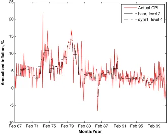
Plots of core inflation
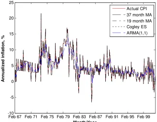
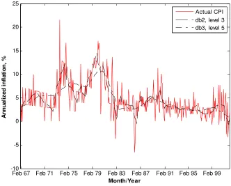
Before carrying out more formal comparisons, it is good practice to plot the various
core inflation series and look for any outstanding features. Plots of our series are
given in Figures 2-6: Figure 2 gives plots of the ‘CPI-ex’ core inflation measures,
Figure 3 gives plots of the regression-based measures and Figures 4-6 give plots of
our chosen wavelets. In each case, we also plot the ‘parent’ CPI inflation rate for
comparison. We separate out the wavelet plots so that Figure 4 gives plots of the two
‘smooth’ wavelet measures, Figure 5 gives plots of the ‘pointed’ wavelet measures,
and Figure 6 gives plots of the ‘plateaued’ wavelet measures. A comparison of these
Figures indicates that there are some striking differences between different core
inflation series.
Insert Figures 2-6 here
Evaluation criteria
The performance of core inflation measures can be evaluated using a number of
criteria. As outlined earlier we have two performance criteria for our candidate
27 Because the MA and Cogley measures involve measures of core inflation that involves long lag
23
measures that are based on alternative definitions of core inflation: ability to track a
trend and predict future inflation.
Beginning with trend based evaluation, we might expect a good core
inflation series to have the same mean as its ‘parent’ inflation series (see, e.g., Clark,
2001, Table 2). Moreover, a good core inflation measure should also have a lower
variance than its parent series, and this suggests that the core series should pass a test
of the hypothesis that its variance is less than that of its parent series. A trend-based
notion of core inflation should also lead us to expect that a core inflation series
would exhibit fewer turning points than its parent series. In addition, we might expect
a good measure of core inflation to be cointegrated with its parent inflation series
(e.g., as in Freeman, 1998, Marques et al., 2000), and we might also expect the
difference between these two series to be stationary.
If we think in terms of core inflation as a predictor of future inflation, then
we are looking for evaluation criteria that address the ‘closeness’ between core
inflation now and actual inflation later. This suggests that we might use the variance
of the difference between current core inflation and later actual inflation as an
evaluation criterion: the lower the variance, the better the fit. We might also expect
core inflation now and actual inflation later to be cointegrated, and the prediction
error to be stationary.
We can also examine whether a candidate core inflation series passes a
recent inflation-prediction test suggested by Cogley (2002). If c t
24
(inflation predicting) core inflation, then for any reasonable horizon H, the
regression:
(1) t H c
t t t
H
t+ −π =α+β (π −π )+u+
π
should satisfy the predictions α =0 and β =−1. These restrictions reflect the
expectations that a good core inflation series should predict future changes in
inflation by the right magnitude. So for example, if the slope coefficient is less
(greater) than one in an absolute sense it suggests that the measure of core inflation is
overpredicting (underpredicting) the magnitude of subsequent changes in inflation.
We would also expect the regression to exhibit a good overall fit (e.g., a high R2).
Results28
Table 1 reports summary results for the means, volatilities and the numbers of
turning-points of each core inflation series. These are presented as the relevant core
inflation parameters divided by their parent inflation counterparts:
• Means: Most series have mean ratios indicating that their means are close (or
even identical) to those of the parent CPI series. The accuracy of the wavelet
measures in particular is striking. The only series that perform poorly by this
28 It has been argued that a good core inflation measure should also remove any seasonality in the
25
criterion are the trimmed mean, short MA and exponentially smoothed
measures. These are respectively 8.9%, 6.1% and 7.1% away from their target
of 1 whereas the other ratios are generally within 1% of the target ratio.
• Variances: The CPI-ex measures have very variable variance ratios, ranging
from 0.386 (18% trimmed mean) to 0.948 (CPI less food). The
regression-based ratios tend to be lower and vary from 0.295 (exponentially smoothed) to
0.509 (short MA). The wavelet ratios tend to be in-between the others and vary
from 0.420 (db3, level 5) to 0.663 (Haar, level 2).
• Numbers of turning points: The CPI-based measures clearly perform badly by
this criterion, as their turning point ratios all exceed 1. The regression-based
measures perform better with turning point ratios varying from 0.542 to 0.792,
and the wavelet-based measures perform much better still with ratios varying
from 0.064 to 0.441.
Insert Table 1 here
These results indicate that CPI based measures tend to perform poorly
across one or more criteria – the trimmed mean, short MA and exponentially
smoothed measures do badly by the mean criterion, CPI-less-food does badly by the
variance criterion, and the CPI-ex measures all do badly by the turning point
26
criterion. The performance of the regression-based measures is mixed, and that of the
wavelet-based measures is pretty good.29
Results for the tests of cointegration between core and parent inflation
series are presented in Table 2. These give a clear picture: all the results reported
indicate that the relevant pairs of series are cointegrated.
Insert Table 2
Results for tests of the stationarity of the difference between core and
parent inflation series are presented in Table 3. For every series, the null hypothesis
of a unit root is easily rejected: all series pass with flying colors. Thus, these first two
tests give us no reason to prefer any one measure of core inflation to any others.
Insert Table 3
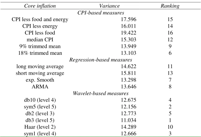
We now turn to the inflation-prediction tests, and Table 4 gives the
variances of core inflation prediction errors applied to an 18-month forecast
29
As an aside, note that we have compared each core inflation series to the actual parent series. However, it is quite common in core inflation studies to compare core inflation series to some assumed
27
horizon.30 If we rank them by their lowest-first variance rankings, the CPI-based
measures have rankings varying from 6 to 16 (with most of them at or near the
bottom), the regression-based measures have rankings of 7 to 13, and the wavelets
have rankings from 1 to 10 for the Haar wavelet (and include the top 5 rankings).
Note, too, that the performance of the wavelet measures improves even further if we
exclude the ‘rogue’ Haar wavelet: as Figure 1 shows, this is a fairly ‘primitive’
wavelet anyway. Thus, a fairly clear pecking order emerges: the wavelets generally
perform best by this criterion, and the CPI measures generally perform worst.
Insert Table 4
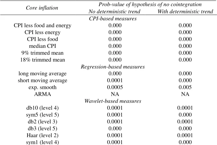
Results for tests of cointegration between core and future parent inflation
series are presented in Table 5.These indicate that the hypothesis of no cointegration
is almost always highly implausible.31
Insert Table 5
Results for tests of the stationarity of the core inflation prediction error are
presented in Table 6, and indicate very clearly that the prediction errors are
stationary.
Insert Table 6
30 We also replicated the prediction results for a 12-month and 24-month forecast horizon. The results
for a 12-month forecast horizon tend to produce very similar rankings; for a 24-month horizon the superiority of the wavelets-based measures over the regression-based ones is still discernable but less marked. These results for prediction errors over alternative forecast horizons are available on request. 31 The results reported in this Table and the next are extremely robust if we change the horizon periods
28
Table 7 gives the prediction results based on estimates of (1). The Table also
reports the individual coefficients of the regression and their standard errors, and
these can be used to carry out t-tests of the two predictions α =0and β =−1
separately considered, and to carry out an F-test of them jointly. We find that the
CPI-based measures fail these tests, the regression-based measures give a mixed
performance, and the wavelet-based measures (usually) perform well. The Table also
reports the different measures’ R2 rankings. The CPI-based measures have the 6
lowest rankings, the regression-based measures have rankings from 4 to 8, and
wavelet-based measures have rankings from 1 to 10 (and include the top 3
performers). A similar pecking order therefore emerges: the wavelets generally
perform best, and the CPI-based measures perform worst, and the regression-based
measures (usually) perform somewhere between.
Insert Table 7 here
If we take all these results together, we can also say something about the
relative performance of individual series in each of these groups:
• CPI-based measures: There is not a great deal to choose from between ‘CPI
less x’ and median CPI measures. Amongst the CPI-based measures, the
trimmed mean measures perform worst in the ratio of means results in Table 1,
but in contrast outperform the other CPI measures in the inflation-prediction
29
• Regression-based measures: There is also little to choose from between most
of these measures, except to point out that the exponentially smoothed measure
performs worst by the ratio of means results in Table 1 but best in the
inflation-prediction results in Tables 4 to 7.
• Wavelet-based measures: Amongst the wavelets, the worst performer is clearly
the Haar measure: this measure is not only the worst wavelet in each ranking,
but its ranking is always well out of the range of the others. Eliminating this
measure would therefore significantly improve the wavelet rankings overall.
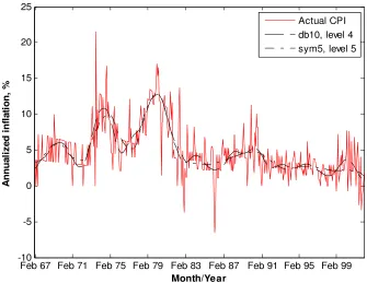
The wavelet results overall also suggest that the ‘smooth’ wavelets generally do
better than the ‘pointed’ ones, which in turn tend to do better than the
‘plateaued’ ones. Thus, our best performers appear to be the ‘smooth’ ones, the
db10 (level 4) and sym5 (level 5), and this makes them very natural measures
of core inflation if we want a ‘smooth’ core inflation series. It is also interesting
to note that these two measures have especially low turning-point ratios –
suggesting the not-unreasonable conclusion that a good measure of (trend) core
inflation should have relatively few turning points.
7. CONCLUSIONS
This paper has suggested using wavelet methods to estimate core inflation. Wavelets
30
estimating core inflation is essentially one of denoising a ‘badly behaved’ time series.
An additional attraction of using wavelets for this purpose is that different wavelets
lead to core inflation series of different shapes, so we can choose a wavelet that
produces the shape we think most appropriate to the precise problem at hand, i.e.,
one which addresses the question of why we want to measure core inflation in the
first place. The paper explains how wavelets might be applied to this purpose, and
sets out a wavelet selection procedure that will generate a core inflation series from
some initial ‘parent’ inflation rate. The paper goes on to compare wavelet-based
measures of core inflation against a number of existing measures, and results indicate
that the wavelet-based measures generally do better, and often much better, than
earlier core inflation measures.32 The performance of the wavelet measures is
particularly impressive, and not least because the wavelets were chosen merely for
illustrative purposes and no effort was made to find an ‘optimal’ wavelet measure.
There is therefore every reason to believe that an ‘optimal’ wavelet would perform
even better.33
32 The choice between different wavelets comes down, in part, to which of these types of trends is most
plausible for the application at hand. However, from the point of view of identifying core inflation as trend inflation, the ‘smooth’ trends are presumably more plausible in this context than the other ones. Interestingly, the two individual wavelets that dominate the performance evaluation are both examples of wavelets that produce ‘smooth’ core inflation series.
33 Two obvious extensions to our work are therefore as follows. (1) How more sophisticated wavelet
31 REFERENCES
Álvarez, L. J., and M. Llanos (1999) “Underlying inflation measures in Spain.”
Proceedings of the Bank for International Settlements Workshop on Measures of
Underlying Inflation and their Role in the Conduct of Monetary Policy. Available at
http://www.bis.org/publ/bisp05_p6.pdf
Apel, M.., and P. Jansson (1999) “A parametric approach for estimating core
inflation and interpreting the inflation process.” Proceedings of the Bank for
International Settlements Workshop on Measures of Underlying Inflation and their
Role in the Conduct of Monetary Policy. Available at
http://www.bis.org/publ/bisp05_p2.pdf
Blinder, A. S. (1997) “Commentary.” Federal Reserve Bank of St. Louis Review
(May-June 1997): 157-160.
Bryan, M. F., and S. G. Cecchetti (1993) “The consumer price index as a measure of
inflation.” Federal Reserve Bank of Cleveland Economic Review (1993:4): 15-24.
Bryan, M. F., and S. G. Cecchetti (1994) “Measuring core inflation”. Pp. 195-215 in
N. Gregory Mankiw (ed.) Monetary Policy. Chicago: Chicago University Press.
Bryan, M. F., S. G. Cecchetti, and R. L. Wiggins, III (1997) “Efficient inflation
estimation.” NBER Working Paper No. 6183.
Cecchetti, S. G. (1997) “Measuring short-run inflation for central bankers.” Federal
Reserve Bank of St. Louis Review (May-June 1997): 143-155.
Clark, T. E. (2001) “Comparing measures of core inflation.” Federal Reserve Bank of
32
Cogley, T. (2002) “A simple adaptive measure of core inflation.” Journal of Money,
Credit, and Banking 34: 94-113.
Coifman, R. R., and D. Donoho (1995) “Time-invariant wavelet denoising.” In
Wavelets and Statistics, Pp 125-150 in A. Antoniadis and G. Oppenheim (eds.)
Volume 103 of Lecture Notes in Statistics, Springer-Verlag, New York.
Cockerell, L., (1999) “Measures of inflation and inflation targeting in Australia”
Proceedings of the Bank for International Settlements Workshop on Measures of
Underlying Inflation and their Role in the Conduct of Monetary Policy. Available at
http://www.bis.org/publ/bisp05_p5.pdf
Daubechies, I. (1992) “Ten Lectures on Wavelets.” Volume 61 of CBMS-NSF
Regional Conference Series in Applied Mathematics, Society for Industrial and
Applied Mathematics, Philadelphia.
Eckstein, O. (1981) Core Inflation. Englewood-Cliffs, NJ: Prentice-Hall.
Freeman, D. G. (1998) “Do core inflation measures help forecast inflation?”
Economics Letters 58: 143-147.
Gabor, D. (1946) “Theory of communication.” Journal of the Institute of Electrical
Engineers, 93: 429-457.
Gençay, R., F. Selçuk, and B. Whitcher (2002) An Introduction to Wavelets and
Other Filtering Methods in Economics and Finance. San Diego: Academic Press.
Hogan, S., M. Johnson, and T. Laflèche (2001) “Core inflation”. Bank of Canada
33
Jensen, M. (1999) “Using wavelets to obtain a consistent ordinary least squares
estimator of the long-memory parameter.” Journal of Forecasting, 18: 17-32.
Johnson, M., (1999) “Core inflation: a measure of inflation for policy purposes.”
Proceedings of the Bank for International Settlements workshop on Measures of
Underlying Inflation and their Role in the Conduct of Monetary Policy. Available at
http://wb-cu.car.chula.ac.th/Papers/bis/inflation04.pdf
Mallat, S. (1989) “A theory of multiresolution signal decomposition: the wavelet
representation.” IEEE Transactions on Pattern Analysis and Machine Intelligence,
11: 674-693.
Marques, C. R., P. D. Neves, and L. M. Sarmento (2000) “Evaluating core inflation
indicators.” Banco de Portugal Working Paper 3-00.
Misiti, M., Y. Misiti, G. Oppenheim, and J.-M. Poggi (2000) Wavelet Toolbox for
Use with MATLAB. Natick, MA: The MathWorks, Inc.
Quah, D., and S. P. Vahey (1995) “Measuring core inflation.” Economic Journal
105: 1130-1144.
Ramsey, J. B., and Z. Zhang (1997) “The analysis of foreign exchange data using
waveform dictionaries.” Journal of Empirical Finance 4: 341-372.
Ramsey, J. B., and Lampart, C. (1998) “The decomposition of economic
relationships by time scale using wavelets: money and income.” Macroeconomic
34
Ramsey, J. B., (1999) “The contribution of wavelets to the analysis of economic and
financial data.” Philosophical Transactions of the Royal Society of London A 357:
2593-2606.
Rich, R., and C. Steindel, (2005) “A Review of Core Inflation and an Evaluation
of Its Measures”, Federal Reserve Bank of New York, Staff Report No. 236.
Roger, S. (1998) “Core inflation: concepts, uses and measurement.” Mimeo. Reserve
Bank of New Zealand.
Roughan, M., D. Veitch and P. Abry (2000) “Real-time estimation of the parameters
of long-range dependence.” IEEE/ACM Transactions on Networking. 8: 467-478.
Schleicher, C. (2002) “An introduction to wavelets for economists.” Bank of Canada
Working Paper No. 2002-3.
Smith, J. K. (2004) “Weighted median inflation: Is this core inflation?” Journal of
Money, Credit, and Banking. 36: 253-263.
Smith, J. K. (2006) “PCE Inflation and Core Inflation?” SSRN
http://ssrn.com/abstract=891142.
Stevenson, M. (2001) “Filtering and forecasting spot electricity prices in the
increasingly deregulated Australian electricity market.” University of Technology,
Sydney, Quantitative Finance Research Papers No. 63.
Vega, J.-L., and M. A. Wynne (2001) “An evaluation of the some measures of core
inflation for the euro area.” European Central Bank Working Paper No. 53.
Wynne, M. A. (1997) “Commentary”. Federal Reserve Bank of St. Louis Review
35
Wynne, M. A. (1999) “Core inflation: A review of some conceptual issues.”
European Central Bank Working Paper Number 5.5.
Wynne, M. A. (2001) “The Edgeworth index as a measure of core inflation.” Mimeo.
36 FIGURES
FIGURE 1: Illustrative Wavelets
0 0.5 1
-2 -1 0 1 2 Haar wavelet v a lu e domain
-5 0 5
-0.5 0 0.5 1
Mexican hat wavelet
v
a
lu
e
domain
0 2 4 6
-1 0 1 2 Db4 wavelet v a lu e domain
0 1 2 3
37
FIGURE 2: CPI-Based Measures of Core Inflation
Feb 67 Feb 71 Feb 75 Feb 79 Feb 83 Feb 87 Feb 91 Feb 95 Feb 99
-10 -5 0 5 10 15 20 25
Month/Year
A
n
n
u
a
li
z
e
d
i
n
fl
a
ti
o
n
,
%
Actual CPI
CPI less food and energy CPI less energy
CPI less food Median CPI 9% trimmed mean 18% trimmed mean
38
FIGURE 3: Regression-Based Measures of Core Inflation
Feb 67 Feb 71 Feb 75 Feb 79 Feb 83 Feb 87 Feb 91 Feb 95 Feb 99 -10
-5 0 5 10 15 20 25
Month/Year
A
n
n
u
a
li
z
e
d
i
n
fl
a
ti
o
n
,
%
Actual CPI 37 month MA 19 month MA Cogley ES ARMA(1,1)
39
FIGURE 4: ‘Smooth’ Wavelet-Based Measures of Core Inflation
Feb 67 Feb 71 Feb 75 Feb 79 Feb 83 Feb 87 Feb 91 Feb 95 Feb 99 -10
-5 0 5 10 15 20 25
Month/Year
A
n
n
u
a
li
z
e
d
i
n
fl
a
ti
o
n
,
%
Actual CPI db10, level 4 sym5, level 5
40
FIGURE 5: ‘Pointed’ Wavelet-Based Measures of Core Inflation
Feb 67 Feb 71 Feb 75 Feb 79 Feb 83 Feb 87 Feb 91 Feb 95 Feb 99
-10 -5 0 5 10 15 20 25
Month/Year
A
n
n
u
a
li
z
e
d
i
n
fl
a
ti
o
n
,
%
Actual CPI db2, level 3 db3, level 5
41
FIGURE 6: ‘Plateaued’ Wavelet-Based Measures of Core Inflation
Feb 67 Feb 71 Feb 75 Feb 79 Feb 83 Feb 87 Feb 91 Feb 95 Feb 99
-10 -5 0 5 10 15 20 25
Month/Year
A
n
n
u
a
li
z
e
d
i
n
fl
a
ti
o
n
,
%
Actual CPI haar, level 2 sym1, level 4
42 TABLES
Table 1: Summary Results for Core Inflation Measures
Core inflation measure Ratio of means Ratio of variances Ratio of turning points CPI-based measures
CPI less food and energy 1.015 0.635 1.114
CPI less energy 1.010 0.643 1.076
CPI less food 1.003 0.948 1.047
median CPI 1.011 0.560 1.140
9% trimmed mean 0.890 0.468 1.106
18% trimmed mean 0.890 0.386 1.110
Regression-based measures
long moving average 1.004 0.381 0.602 short moving average 1.061 0.509 0.542
Exp. Smooth 0.929 0.295 0.593
ARMA 1.000 0.444 0.792
Wavelet-based measures
db10 (level 4) 1.011 0.526 0.072
sym5 (level 5) 0.996 0.498 0.064
db2 (level 3) 0.999 0.560 0.271
db3 (level 5) 0.995 0.420 0.106
Haar (level 2) 1.000 0.663 0.441
sym1 (level 4) 1.000 0.545 0.110
Notes: Ratio of means is mean core inflation divided by mean CPI inflation; ratio of variances is
43
Table 2: Test Results for Cointegration Between Core Inflation and CPI Inflation Series
Prob-value of hypothesis of no cointegration Core inflation
No deterministic trend With deterministic trend CPI-based measures
CPI less food and energy 0.000 0.000
CPI less energy 0.000 0.000
CPI less food 0.000 0.000
median CPI 0.000 0.000
9% trimmed mean 0.000 0.000
18% trimmed mean 0.000 0.000
Regression-based measures
long moving average 0.000 0.000
short moving average 0.0001 0.000
exp. smooth 0.0005 0.005
ARMA NA NA
Wavelet-based measures
db10 (level 4) 0.0001 0.0001
sym5 (level 5) 0.0001 0.000
db2 (level 3) 0.0001 0.0001
db3 (level 5) 0.000 0.000
Haar (level 2) 0.0001 0.0001
sym1 (level 4) 0.0001 0.000
Notes: Results are based on 415 observations over 67:7 to 02:1. Results are for the Johansen
44
Table 3: Stationarity Test Results for Difference between Core Inflation and CPI Inflation Series
Aug. Dickey-Fuller statistic Core inflation
No intercept With intercept
CPI-based measures
CPI less food and energy -11.616** -11.611** CPI less energy -18.789** -18.775**
CPI less food -13.075** -13.059**
median CPI -17.047** -17.033**
9% trimmed mean -10.653** -16.194**
18% trimmed mean -10.423** -11.009**
Regression-based measures
long moving average -6.379** -6.372** short moving average -9.532** -9.608**
exp. Smooth -7.126** -7.211**
ARMA -18.890** -18.867**
Wavelet-based measures
db10 (level 4) -18.113** -18.091** sym5 (level 5) -16.611** -16.593**
db2 (level 3) -12.788** -12.773**
db3 (level 5) -14.287** -14.272**
Haar (level 2) -14.489** -14.471** sym1 (level 4) -18.086** -18.065**
Notes: ** = significant at 1% level. Test statistic is distributed as a t. Results are based on 419
45
Table 4: Variances of Core Inflation Prediction Errors
Core inflation Variance Ranking
CPI-based measures
CPI less food and energy 17.596 15
CPI less energy 16.011 14
CPI less food 19.422 16
median CPI 15.303 12
9% trimmed mean 13.949 9
18% trimmed mean 13.103 6
Regression-based measures
long moving average 14.622 11
short moving average 15.811 13
exp. Smooth 13.298 7
ARMA 13.646 8
Wavelet-based measures
db10 (level 4) 12.675 4
sym5 (level 5) 12.156 2
db2 (level 3) 12.773 5
db3 (level 5) 11.034 1
Haar (level 2) 14.289 10
sym1 (level 4) 12.666 3
Notes: Results are based on 402 observations over 68:8 to 02:1, with an assumed forecast
horizon of H=18 months. The prediction error is the difference between core inflation and
46
Table 5: Test Results for Cointegration Between Core Inflation and Future CPI Inflation Series
Prob-value of hypothesis of no cointegration Core inflation
No deterministic trend With deterministic trend CPI-based measures
CPI less food and energy 0.0001 0.0001
CPI less energy 0.0000 0.0000
CPI less food 0.0003 0.0002
median CPI 0.0000 0.0000
9% trimmed mean 0.0004 0.0011
18% trimmed mean 0.0003 0.0014
Regression-based measures
long moving average 0.0027 0.0306
short moving average 0.0003 0.0037
exp. Smooth 0.0006 0.0094
ARMA 0.0002 0.0012
Wavelet-based measures
db10 (level 4) 0.0001 0.0000
sym5 (level 5) 0.0000 0.0000
db2 (level 3) 0.0000 0.0001
db3 (level 5) 0.0000 0.0000
Haar (level 2) 0.0000 0.0002
sym1 (level 4) 0.0000 0.0000
Notes: Results are based on 397 observations over 67:7 to 00:4 with an assumed horizon of 18
47
Table 6: Stationarity Test Results for Core Inflation Prediction Error
Aug. Dickey-Fuller statistic Core inflation
No intercept With intercept
CPI-based measures
CPI less food and energy -7.485** -7.483**
CPI less energy -8.049** -8.045**
CPI less food -4.222** -4.225**
median CPI -7.542** -7.535**
9% trimmed mean -4.213** -4.232**
18% trimmed mean -5.640** -5.686**
Regression-based measures
long moving average -4.776** -4.774** short moving average -4.599** -4.629**
exp. Smooth -5.061** -5.063**
ARMA -5.144** -5.140**
Wavelet-based measures
db10 (level 4) -5.322** -5.322**
sym5 (level 5) -5.473** -5.471**
db2 (level 3) -5.466** -5.466**
db3 (level 5) -5.854** -5.853**
Haar (level 2) -5.780** -5.780**
sym1 (level 4) -5.587** -5.845**
Notes: Results are based on 418 observations over 67:4 to 02:1 with an assumed forecast
horizon of H=18 months. The prediction error is the difference between core inflation and
48
Table 7: Prediction-based Test Results for Core Inflation Measures
Core inflation measure
Intercept Slope F-test prob
R2 R2
ranking CPI-based measures CPI less food and energy -0.121
(0.371) (0.064) -0.519 0.000 0.352 14
CPI less energy -0.106 (0.338) -0.464 (0.081)
0.000 0.305 15
CPI less food -0.099 (0.375) -0.353 (0.088)
0.000 0.275 16
median CPI -0.074 (0.058) -0.685 (0.069)
0.000 0.393 13
9% trimmed mean -0.393 (0.362) -0.875 (0.070)
0.090 0.456 12
18% trimmed mean 0.416 (0.349) -0.887 (0.065)
0.084 0.483 11
Regression-based measures long moving average -0.085 (0.410) -0.872 (0.053)
0.057 0.537 6
short moving average
-0.317
(0.454) (0.055) -0.890 0.102 0.527 8
exp. smooth 0.250 (0.382) -0.898 (0.054)
0.130 0.545 4
arma -0.075 (0.389)
-0.791 (0.043)
0.001 0.538 5
Wavelet-based measures db10 (level 4) -0.101 (0.371) -0.910 (0.055)
0.004 0.547 3
sym5 (level 5) -0.082 (0.354) -0.910 (0.054)
0.177 0.552 2
db2 (level
3) (0.372) -0.101 (0.055) -0.900 0.184 0.512 9 db3 (level
5) (0.317) -0.088 (0.053) -0.911 0.239 0.563 1 Haar (level 2) -0.101 (0.388) -0.808 (0.058)
0.246 0.486 10
sym1 (level 4) -0.090 (0.363) -0.897 (0.056)
0.250 0.534 7
Notes: First numbers in second and third columns are estimated parameters; numbers in
49