Optimal Wiring on Rectangular Structure
Pawan Kumar Patel
Department of Computer Science and Engineering Indian Institute of TechnologyKanpur, India
Rohit Kumar
Department of ElectricalEngineering
Indian Institute of Technology (BHU) Varanasi, India
Nikita Gulati
Department of Computer Science and Engineering Lucknow Model Institute of Technology Lucknow, IndiaABSTRACT
In this paper we worked upon on optimal wiring on rectangular structure. Here we are given a rectangle partitioned into smaller rectangles by axis-parallel line segments. Find a subset of the segments such that the resulting structure from these segments is connected and it touches every smaller rectangle.
Here we reduce the problem of exact cover by 3-sets (X3C), which is known to be NP-complete, into this problem and thus claim wiring problem to be NP-hard. This problem carries a special importance because very few problems in the domain of geometry are known to be NP-hard.
Keywords
Wiring on rectangular structure, NP-hard, Computational geometry, Graph theory
1.
INTRODUCTION
Given a rectangle partitioned into smaller rectangles by horizontal and vertical line segments, find a set of the line-segments which touches each rectangle at least at one point on its boundry and these segments are connected (i.e., there is a path between any two points of these segments ). The optimization criterion is to minimize the sum of lengths of these segments.
An obvious application of this problem is to how to wire a building using minimum wire. Same applies to laying cooling or heating channels. Another application is in connecting modules of a VLSI chips.
2.
NP_HARDNESS Of WIRING
PROBLEM
2.1. Wiring Problem
A floorplan is a rectangle in a plane which is partitioned by horizontal and vertical line segments such that each region is also a rectangle. For convenience treat it as a graph where the vertex set is the collection of the corners of all the rectangles and edges are the line segments between the vertices in the floor plan. A side is a line segment which connects two corners of the same rectangle. In general a side may contain more than one edge.
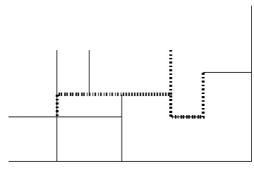
[image:1.595.329.509.226.352.2]The wiring problem is to compute a minimum length connected subgraph of a floorplan (i.e., total length of the edges of the subgraph be minimum) which contains at least one vertex on the boundry of every rectangle. Observe that it will always be a tree. See figure 1. In this section we shall show that this problem is NP-hard by reducing 3-set-exact-cover problem. The proof is adapted from the proof of hardness of steiner tree computation for geometric rectilinear graph by Garey, Graham, and Johnson[1].
Figure 1: A floorplan and its solution
2.2 3-set-Exact-Cover (X3C) Problem
Given a family, F= {F1, F2,…..Ft}, of 3-element subsets of a universal set U of 3n elements, decide if there exists a subfamily F’ Ϲ F of pairwise disjoint sets such that the union of all members of F’ is equal to U. This problem is NP_complete[2]. We will prove the hardness of the wiring problem by transforming X3C into it.2.3 The overall plan
Let F= {F1, F2,…..Ft} be an input to the X3C (3-set exact cover) problem, where the universal set is assumed to be the integer set {1, 2,……,3n}, we will construct a floorplan Pi associated with set Fi for each i. Each plan will be of the same dimensions. Then we shall join them side by side along the X-axis to form a single floor-plan P for the given F.
We will show that there is a polynomial L(n,t) such that the length of the wiring tree for P will be less than or equal to L(n.t) if and only if the given F has an exact cover. It will also be shown that an exact cover can be extracted from such a solution tree in O(L(n,t)) time.
2.4. Construction of Pi
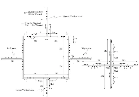
We first introduce two gadgets, junction and crossover, which are the bulding blocks of the floor-plans Pi. Figure 1 shows the gadgets. There are two variants of crossover, standard and warped. The length parameters used in describing the gadgets are K = 162qnt + 2888n2t _ 9n + 1 and ϵ which will define later. It will be helpful to remember that ϵ <<1.
Symbol q is defined to be sum of (ai + bi +ci) for i= 1 to t, where Fi = {ai, bi, ci}.
Each junction has one and each crossover has two active regions which are highlighted by shading in figure 1.
Each stack has one warped crossover at the top and remaining crossovers are standard. The width of Pi is 24K and the height
[image:2.595.69.541.97.426.2]is 24nK + 8K + ϵ.
Figure 2: Crossover and Junction
The floorplan P associated with F is constructed by placing P1, P2,………,Pt side by side so that right side of Pi coincides
with the left side of Pi+1. In addition, a stack is attached to the
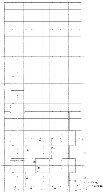
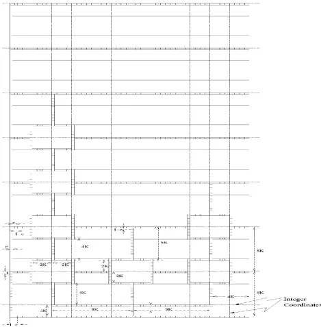
left of the figure consisting of 8K rectangles of size 1x ϵ and one 24nK xϵ rectangle at the top of the stack, see figure 4 for P1 with the additional stack at the left wall. One way P1 and Pt
differ from other Pi is that the leftmost rectangles in the
horizontal chain of small rectangles in P1 end with an ϵ x ϵ
rectangle. This is the case for all but the bottom two chains. In case of Pt the rightmost rectangles of all but the bottom chain
is ϵ x ϵ. Figure 5 shows complete P. It uses q crossovers and t junctions.
2.5 Optimal wiring tree for P
In this section we will determine some properties of any optimal solution of the wiring on P which are crucial for the proof. In the following section we use these properties to show that the sum of the lengths of the edges in the optimal solution, will be less than or equal to L(n.t) if and only if the underlying X3C problem has a solution.
2.5.1 Coverage of the smaller rectangles
Let us partition the rectangles of P into 3 classes: R0 which
have longer side upto 1 + ϵ; R1 which have longer sides in the
range from 54nt -1 to 72nt; and R2 have each side at least
2K-ϵ in length. This partitions all rectangles of P except the top rectangle at the left boundry. This ϵ x24nK rectangle is also included in class R2. Observe that R1 are precisely the
rectangles in the active regions. We further partition R0 into
terminal and non terminal rectangles, where the former contains all the ϵ x ϵ sized rectangles. Observe that at least one
vertex of each smaller side of a no-terminal rectangle is shared by other R0 rectangles. We shall denote these subclass
by R0t and R0n respectively. Terminal rectangles are attached
to the left side of P1, right side of Pt, and to each R1 rectangle.
In the similar fashion as for the rectangles partition the edges also into 3 classes: E0 consists of edges of length not
exceeding 1 + ϵ; E1 are the edged with length between 54nt-1
to 72nt; and E2 have all the larger edges. Verify that each edge
of E2 is longer than K.
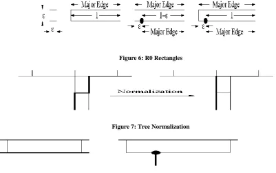
In order to establish polynomiality of this transformation from X3C, we need to determine some counts. Break the R0n class
into four subclasses, see figure 6, and denote the number of (i) 1 xϵ rectangles with 4 vertices by m1, (ii) those with 5
vertices by m2, (iii) (1- ϵ ) x ϵ sized rectangles by m3, and (iv)
(1 + ϵ ) x ϵ sized rectangles by m4. The number of terminal
rectangles will be denoted by m0. A trivial but cumbersome
exercise gives m0 = 6q + 6n + 4t + 1, m1 = 14Kq + 42Kt +
72Kn + 65K -324qnt – 288nt2 -10t +q –n -1, m2 = 2q + 5t + 1,
m3 = 6n +7t + 8q + 1, and m4 = 4q + t + 1. Since q<9nt, each
of these numbers is a polynomial in n, t. Each R0n rectangle
has two major edges which are parts of the longer sides and which have length between 1- ϵ and 1+ ϵ .
In this paper we adopt a convention in which the same symbol will represent a set of edges as well as the graph induced by those edges, depending on the context.
Henceforth P will denote the complete floorplan with ϵ = 1(20q + 23n +28t +9).
T0 will denote T∩ E0 and T1 = T-T0. Observe that the residue
of each R0 rectangle in P’ is an edge of length 1. By T’ denote
limϵ→0 T. Similarly by T’0 and T ’
1 denote the residue of T0 and
T1 in P’.
Observation 1 Every cycle in P has at least one edge of size greater than ϵ.
Observation 2 Each cycle in P’ contains an edge which is the residue of the longer side of an R1 rectangle, i.e., an active
region rectangle.
Observation 3 There are 4q + 8t + 9n + 2 rectangles and each of these rectangles has at least one R0n rectangle adjacent to it. Proposition 4 Let X be an R0 rectangle and C be a cycle in P.
Let C contain a major edge e of X which is contained in side s. Let s’ be the side parallel to s in X. Then (i) s is a longer side of X, (ii) either C contain s’ or it contains a longer side of an R1 rectangle.
Proof (i) Major edges are contained in the longer sides of a rectangle.
(ii) As we take the limit limϵ→0, line segments e, s, and s’ will
coincide with a single segment, say s’’ in P’. Let C reduce to C’ in P’. Then the edges of C’ can be partitioned into simple cycles and simple paths. If s’’ is in a simple path, then s’ must be on C. On the other hand, If s’’ is in a cycle in C’, then due to the previous observation the longer side of an R1 rectangle
must be on C.
Lemma 5 T contains at least one major edge from each R0n
rectangle.
Proof Let X be a non terminal rectangle of R0 which does not
satisfy the claim. By the definition,, X has two adjoining R0
rectangle which are separated by more than ϵ. Label them by Y and z. Since T touches all three rectangles, Y’ = T ∩ (Y U X) and Z’ = T ∩ (ZUX) are non-empty where the X, Y, Z may be treated as the sets of the edges on their sides. Since T does not contain any major edge of X, Y’ and Z’ must be unconnected. Let y belongs to Y’ and z belongs to Z’ be a pair of vertices which are closest to each other.
Add the shortest path between y and z in P, to T. Let the resulting subgraph be called H. This added path must contain a major edge e of X and the length of the path canot exceed 3x(1 + ϵ ) + ϵ since sides of each rectangle is at most 1 + ϵ and their width is ϵ. The subgraph H has a cycle (since T is a tree) and the cycle contains e. From proposition 4 either T contains one major edge of X or one longer side of a R1 rectangle. The
former is not possible from the assumption. Therefore T must contain a longer edge p of an R1 rectangle. By deleting p from
H we again get a tree, call it H’, and it also touches all the rectangles. Therefore this is also a candidate of wiring solution. Since the length of p is at least 54nt – 1 and the added edges are at most 3 + 4c in length, H’ has lesser length. This implies that T is not an optimal solution, which is contradiction.
In a wiring solution if a wire connects diagonally opposite vertices of a rectangle then it has two options of equal cost first horizontal then vertical side or its converse. This way we can delay a traversal along an ϵ edge on a non-terminal rectangle until a 5-vertex rectangle is reached. Call such wiring solution normalized, see figure 7. Using this observation and lemma 5 we have following result.
Corollary 6 The cost of T0 is between L0 = m1 + m4 + (1- ϵ)
(m2 + m3) and L0 + ϵ(28q + 21n + 28t + 8).
Proof The smaller major edge of five vertex 1 x ϵ is 1 - ϵ long. The smaller major edge of a (1 + ϵ ) x ϵ rectangle has length 1. Using these fact and the lemma we directly get the lower bound. For the upper bound first delete all the ϵ edges which are pendants ( having one vertex of degree 1 ) from T0. As
observed earlier, the reduced graph can be transformed into normalized from without any extra cost. So assume that the reduced T0 is normalized.
Then the cost due to five vertex rectangles can be upto 1 + ϵ for 1 x ϵ rectangle and 1 + 2 ϵ for (1 + ϵ )x ϵ rectangles. In addition the solution may cover terminal rectangles. So the cost can increase upto 2 ϵ(m0 + m2 + m4). To this we add the
cost of the pendants. The only purpose for the pendants will be to touch the R2 rectangles as all others are already in
contact of T0. This can add at most 4q + 8t + 9n + 2 ϵ edges to
T0.
Observation 7 The graph induced by R0 rectangles has 2q +
3n +1 connected components.
This observation and lemma 5 imply that the subgraphs induced by T0 must have at least 2q + 3n + 1 components. Lemma 8 T0 has exactly 2q + 3n +1.
Proof Assume that the number of components is greater than 2q + 3n +1. Then there must be at least two components of T0
in the same component of R0.
Consider two such T0 components. If there is a R0n rectangle
in this component such that each of its major edge belongs to some T0 component. Then these T0 components are separated
by ϵ distance. In case no R0n rectangle contributes its major
edge to more than one component, then there must be a rectangle whose one vertex is touched by one T0 component
and one major edge belongs to another, see figure 8. Sice the distance between a vertex and a major edge is at most 2 ϵ (in a 5 vertex rectangle), the two components are separated by a path of at most 2 ϵ length. In other words, their closest points are separated by a path of at most 2 ϵ length. Add this path to T, which will create a cycle. Delete a non- ϵ -edge from this cycle. The resulting tree connects the same set of vertices (or one more) as does T therefore it is also a candidate solution for the wiring problem. This tree costs lesser than T since 2 ϵ < 1- ϵ. but this is not possible since T is optimal.
Corollary 9 There is one T0 component in each R0
component.
Lemma 10 T’ has no cycles.
Proof We know that T is a tree. Assume that T’ has a cycle. Then T must have two vertices which are separated by a path S of ϵ-edges which is not a part of T. The longest such path in P has length 2 ϵ. Then T U S will have a cycle which contains S. Once again, as in the proof of Lemma 8 we can construct another solution of the wiring problem which costs less. Therefore the assumption must be wrong.
2.6 Connecting the components of T0
In this section we will establish the underlying X3C problem has an exact cover if and only if T costs less than L = L0 +
time solution, then X3C can also be solved in polynomial time since L is a polynomial in n, t.
In order to construct the solution tree we need to include the edges in addition to T0 so that the resulting graph becomes
connected. Denote the set of these edges by T1. Irrespective of
any other criterion/consideration these edges must provide connections between 2q + 3n + 1 components of T0 graph.
The additional edges will be from E1 U E2. Each E2 edge is at
least K in length. We will show that this renders it too expensive to use. The T1 edges belonging to an active region
become responsible to connect the T0 component surrounding
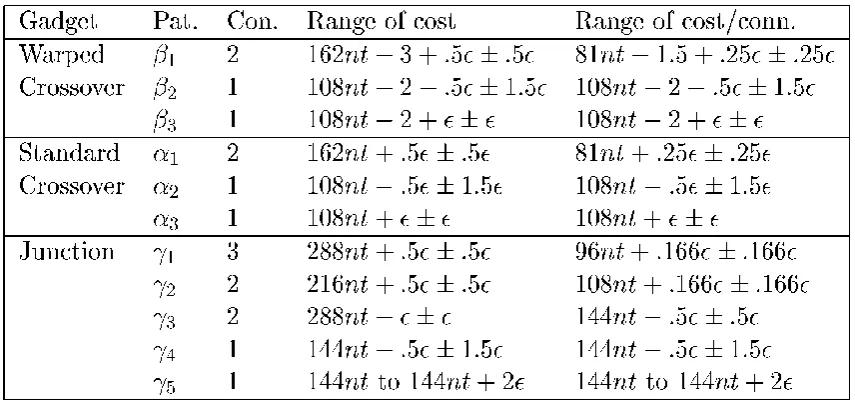
the region. Therefore these edges from 1 or 2 connections, depending upon whether they connect 2 or 3 components. Figure 9 shows possible patterns of these T1 edges. Table 1
[image:4.595.63.491.219.421.2]shows the average cost of forming one connection under these patterns.
Table 1: Patterns for active region, number of connections and their costs
Lemma 11 If T1 Ϲ E1 then (i) the number of α1 and β1
patterns cannot be more than q.
(ii) if the number of α1 and β1 patterns is equal to q, then the
number of β1 patterns cannot be more than 3n.
Proof (i) If there are more than q patterns of α1 and β1 type,
then at least one crossover will have two α1’s or one α1 and
one β1 (in case of top of the stack crossovers). Then T’ will
have a cycle, contradicting Lemma 10.
(ii) If q connection of the type α1 and β1 are used, then each
crossover will have one of these connections, because as shown in part (i) same crossover cannot have two of these connections. This will connect all the chains of the same level. If more than 3n β1-connections are used, then some level will
have two or more connections. This will provide more than one connection between the horizontal chain of that level and that of the level immediately above. Once again it implies that T’ has a cycle.
Lemma 12 Let T1 Ϲ E1. If in a wiring tree the cost of T1 is
less than 162qnt + 288n2t -9n + 1, then the T1 will have 3n
patterns of β1 type, q-3n patterns of α1 type and n patterns of
γ1 type.
Proof Suppose in the given solution u connection (between a pair of T0 components) are due to β1 patterns, v connections
are from α1 patterns w connection from γ1 patterns and
remaining 2q + 3n –u-v-w connections due to other patterns. Then from the table 1 T1 must cost off at least (81nt-1.5)u +
(81nt)w + (108nt) (2q+3n-u-v-w). We are given that this cost
is less than 162qnt + 288n2t – 9n + 1. Simplifying the inequality we get (2q + 3n –u –v-w)12nt + (2q-u-v)15nt + 9n – 1.5u -1 <0. Sice there can be at most 3t patterns of β1 type,
u≤6t. Thus 15nt > 12nt > 1.5u + 1. Lemmas 8 and 11 shows that 2q + 3n-u-v-w and 2q-u-v are non negative. If either of these quantities is positive then the left hand side expression will become positive. This requires that 2q + 3n –u –v –w =0 and 2q –u -v =0. Then inequality simplifies to 1.5(6n –u) -1 < 0. As 2q- u –v =0, from Lemma 11 we also know that 6n-u ≥ 0. Again observe that if 6n –u is positive then this inequality will be unsatisfiable. So we must have 6n – u =0. So u=6n, v=2q-6n and w= 3n.
Corollary 13 If T1 Ϲ E1 and T1 costs less than 162qnt + 288
n2t -9n +1 , then X3C problem has an exact cover.
Proof We have seen that T1 consists of 3n patterns of β1 type,
q-3n patterns of α1 type, and n patterns of γ1 type. As we have
seen in the proof of Lemma 12 that every crossover has one β1
or α1 pattern. This ensures that the T0 components on
horizontal arms of the same level are connected. If β1 patterns
are at the same level, say i, then there are two connections between levels i and i + 1 (above i). This will lead to a cycle in T’ which is not possible. So each β1 must be at a different
level. This ensures that each level is connected to the upper level through the upper arm of a warped crossover.
Now we will argue that in any stack of crossovers either all active regions contributing to T1 are upper ones or all are
lower ones. Suppose crossover C2 is directly above crossover
active region of C1 share edges with T1. This will render the
T0 component I the vertical arm between the two
disconnected. In case the lower active region of C2 and the
upper active region of C1 contribute edges to T1, then this will
provide a connection between the two levels. In addition, the β1 patterns at the level of C1 crossover also provides a
connection between the same levels. This implies that T’ will have a cycle, which is not possible.
Next we will show that β1 patterns can occur only on those
stacks which are associated with the junction having γ1
pattern. Suppose the top crossover of a stack has β1 where the
corresponding junction does not have γ1. Then that junction
does not contribute any edge to T1 This implies that the
vertical arm of the junction corresponding to the stack remains unconnected since the stack above it will have upper active region with α1 (or β1 ) pattern.
Therefore all β1 pattern must be associated with only the
stacks of junctions with γ1 patterns. Since each β1 pattern is at
a different level, the sets corresponding the junctions having γ1 patterns from an exact cover.
Now we are equipped to prove the main result.
Theorem 14 The underlying X3C problem has an exact cover iff the wiring tree of the corresponding floorplan has a solution costing less that L0 + 162 qnt + 288n2t -9n + 1. Proof (only if ) In Corollary 6 we have seen that a T0 can be
constructed which touches all the rectangles, has 2q + 3n + 1 components and costs L0 + ϵ(28q + 21n + 28t + 8). We
construct T1 as follows.
Let us denote the junction of Pi by Ji. Let the exact cover be F’
= { Fa1,………….,Fan}.
Then a wiring tree can be formed by constituting T1 with : β1
pattern in every top crossover of all the three stacks of Jai for
all Fai for all Fai belongs to F’ , α1 pattern in the upper active
regions of all the standard crossovers of these stacks; α1
patterns in the lower active regions in all the other crossovers; and γ1 pattern on every Jai for all Fai belongs to F’. Total cost
of T1 will be no more than 3n(162nt + ϵ -3) + (q -3n)(162nt +
ϵ) + n(288nt + 2 ϵ). It simplifies to 162qnt + 288n2
t -9n + ϵ (q+2n). The total cost of T is at most L0 + 162qnt + 288n2t-9n
+ ϵ(29q + 23n + 28t +8) which is less than L.
(if) suppose the optimal wiring tree costs less than L. From corollary 6 we know that T0 costs at least L0 so T1 must cost
less than 162qnt + 288n2t-9n +1. From corollary 13 we know that the X3C problem must have an exact cover.
Corollary 15 If wiring problem is in class P, then X3C is also in class p.
Proof Since floorplan has a polynomial number of edges (in terms of n and t), it is possible to verify in O(|T|) time whether there are 3n patterns of β1 type, 2q-3n patterns of α1 type, and
n patterns of γ1 type. Also identify which junctions have the
γ1 patterns in the process. As we consequence we can
construct an exact cover.
Figure 4: Floorplan of p1 with stack of rectangles and terminals at the left
[image:7.595.116.466.563.688.2]Figure 6: R0 Rectangles
[image:8.595.86.453.374.564.2]Figure 7: Tree Normalization
Figure 8: Two T0- components at the same R0 Rectangles
Figure 9 : Active region connection Patterns
3.
CONCLUSION
In this paper we shows that wiring on rectangular floorplan is NP- hard problem by converting it into well known exact 3 cover (X3C). Due to wider application of this problem discuss above lead to think us, is there any good approximation algorithms that give good bound for this problem..
4.
REFERENCES
[1]. M.R. Garey, R. L. Graham, and D.s. Johnson. Some np-complete geometric problems. In STOC 76 : Proceeding of the eighth annual ACM symposium on theory of computing, page 10-22, New York, NY, USA, 1976. ACM Press.
[2]. R.M Karp. Reducibility among combinatorial problems. R. E. Miller and J. W. Thatcher, Plenum press, New York, USA, 1972.
[3]. S. Aaronson. Is P versus NP formally independent? Bulletin of the European Association for Theoretical Computer Science, 81, Oct. 2003