A New Iterative Method for Multi Moving Boundary Problems Based Boundary Integral Method

(1)

http://dx.doi.org/10.4236/jamp.2015.39140

How to cite this paper: Al-Swat, K.K. and Ahmed, S.G. (2015) A New Iterative Method for Multi-Moving Boundary Problems Based Boundary Integral Method. Journal of Applied Mathematics and Physics, 3, 1126-1137.

http://dx.doi.org/10.4236/jamp.2015.39140

A New Iterative Method for Multi-Moving

Boundary Problems Based

Boundary Integral Method

Kawther K. Al-Swat, Said G. Ahmed

*

Department of Mathematics and Statistics, Faculty of Science, Taif University, Taif, Kingdom of Saudi Arabia

Email: *_{[email protected]}

This work is licensed under the Creative Commons Attribution International License (CC BY).

http://creativecommons.org/licenses/by/4.0/

Abstract

The present paper deals with very important practical problems of wide range of applications. The main target of the present paper is to track all moving boundaries that appear throughout the whole process when dealing with multi-moving boundary problems continuously with time up to the end of the process with high accuracy and minimum number of iterations. A new numerical iterative scheme based the boundary integral equation method is developed to track the moving boundaries as well as compute all unknowns in the problem. Three practical applications, one for vaporization and two for ablation were solved and their results were compared with finite ele-ment, heat balance integral and the source and sink results and a good agreement were obtained.

Keywords

Multi-Moving Boundary Problems, Vaporization Problem, Ablation Problem, Source and Sink Method, Finite Element Method, Heat Balance Integral Method, Boundary Integral Method

1. Introduction

The differential equation in a certain domain satisfying some given conditions is referred to as boundary-value problem. If one or more of the boundaries are not known and moving with time, the problem then is referred to as moving boundary problem [1] [2]. Furthermore, if the governing equation is time independent as well as the boundary condition, then the problem is referred to as free boundary problem [3]. Phase change problems are practical examples of free and moving boundary problems, frequently appear in industrial process and other problems of technological interests such as the determination of the depth of the frost or thaw penetration,

(2)

signing of the roadway or other engineering works in cold regions and the so-called re-entry problem of hyper-sonic missiles in aeronautical science [4] [5]. When a body is exposed to heat flux the surface of the body changes phase, the changed phase is immediately removed upon formation. This is referred to ablation problem [6]. A major difference between Stefan and ablation problems is that the overall domain in Stefan problem re-mains fixed in space while the domain in the ablation problem is variable and diminishes in size with time. Nu-merical methods become more popular rather than analytical methods. Some of famous nuNu-merical methods are finite differences [7], finite elements [8], boundary elements [9] and more recent mesh-less (mesh-free) numeri-cal methods [10]. In many aspects, the boundary integral equation method for solving boundary value problems proves to be advantageous over the conventional numerical methods. The present paper deals with very impor-tant practical problems of wide range of applications. The main target of the present paper is to track all moving boundaries that appear throughout the whole process when dealing with multi-moving boundary problems con-tinuously with time up to the end of the process with high accuracy and minimum number of iterations. A new numerical iterative scheme based the boundary integral equation method is developed to track the moving boundaries as well as compute all unknowns in the problem.

2. Mathematical Model

A semi-infinite solid initially at uniform temperature with the following constraints, there is no sub cooling, no mushy zone, solid and liquid phases have equal and constant properties and finally no convection. The mathe-matical formulation consists of three different stages as follow:

Heating stage

( )

2

, 1 ,

, 0

u x t u x t

x t

x α

∂ ∂

= < < ∞

∂

∂ (1)

( )

, 0 i

u x =u (2)

( )

0,

( )

u t q t

x K

∂

= −

∂ (3)

( )

, x

( )

, i

u x t _→∞=ut =u (4) As x=0 reaches the melting temperature, the second stage starts appearing.

Liquid-solid stage

( )

_{( )}

2

1 2

, 1 ,

, 0

u x t u x t

x s t t

x α

∂ ∂

= < <

∂ ∂

  ₍₅₎

( )

0,

( )

u t q t

x K

∂

= − ∂

 ₍₆₎

( )

_{( )}

2

1 2

, 1 ,

,

s s

u x t u x t

s t x

t

x α

∂ ∂

= < < ∞

∂

∂ (7)

( )

,

( )

,

s x s i

u x t _→∞=u t =u (8)

( )

, ₁_{( )}

( )

, ₁_{( )}

s x s t x s t m

u x t ₌ =u_ x t ₌ =u (9)

( )

1

( )

_{( )}

1

, , d

, d s

s m

u x t u x t s t

K K L x s t

x x ρ t

∂ ∂

− = =

∂ ∂



 (10)

Gas-liquid-solid stage

( )

_{( )}

2

2 2

, 1 ,

, 0

v v

u x t u x t

x s t t

x α

∂ ∂

= < <

∂

∂ (11)

( )

_{( )}

2

2 1

2

, 1 ,

,

u x t u x t

s t x s t

t

x α

∂ ∂

= < <

∂ ∂

 

(3)

( )

_{( )}

2

1 2

, 1 ,

,

s s

u x t u x t

s t x

t

x α

∂ ∂

= < < ∞

∂

∂ (13)

( )

, ₁_{( )}

( )

, ₁_{( )}

s x s t x s t m

u x t ₌ =u_ x t ₌ =u (14)

( )

, v

( )

, V

u_ x t =u x t =u (15)

( )

2 d d v v v s t u u

K K L

x x ρ t

∂ ∂

− =

∂ ∂



 (16)

( )

, s

( )

, m

u_ x t =u x t =u (17)

3. Boundary Integral Formulation

Starting by the weighted residual statement for diffusion equation as follows:

(

)

2

* 2

0

, ; , d d 0

u u

k u x t t

t x τ

ξ τ

Ω

 ∂ ₋∂  _{Ω =}

 _∂ 

∂

 

∫ ∫

(18)

In Equation (18) u*

(

ξ τ, ; ,x t

)

is the fundamental solution for diffusion equation and it is defined as:

(

)

(

)

( )

(

)

2

* 1 ,

, ; , exp

4 4π

r x

u x t

k t k t

ξ

ξ τ

τ

  = − ₋ 

− _ _ (19)

In which, r2

( )

ξ

,x =X

( )

ξ

−X x

( )

and X

( )

ξ is the source point while X x

( )

is the field point. Integrating equation (18) twice by parts leads to:

(

)

(

)

(

)

₍

₎

2 * 2 0

2 * *

* 2

0 0

, ; , d d

, ; , , ; ,

d d , ; , d d 0

u u

k u x t t

t x

u x t u x t

k u t k q x t u t

t x

τ

τ τ

ξ τ

ξ τ ξ τ

ξ τ

Ω

Ω Γ

 ∂ ₋∂  _Ω

 _∂ _∂ 

 

 ∂ ∂ 

= _ + _ Ω − Γ =

∂ ∂  

∫ ∫

(20)

For one-dimensional problems, Equation (20) takes the following form:

(

)

(

)

₍

₎

2 * *

* 2

0 0 0 0

, ; , , ; ,

d d , ; , d d 0

u x t u x t

k u x t k q x t u x t

t x

τ _{ξ τ} _{ξ τ} τ

ξ τ  ∂ ∂  + − =    _∂ _∂   

∫ ∫



∫ ∫

 (21)

In Equation (21)

(

)

(

)

2 * *

2

, ; , , ; ,

i

u x t u x t

k

t x

ξ τ ξ τ

δ

∂ ∂

+ = −

∂

∂ (22)

* *

iu u

δ

− = − (23)

Making use of Equations (22) and (23) into Equation (20), the last one takes the following form:

(

)

( ) (

)

* *

0 0 0

, ; , d d , , ; , d 0

k u x t q x t u x t u x t x τ

ξ τ ξ τ

−

_{∫ ∫}

 −

_∫

= (24)

For any point the integral equation takes the following form:

( )

( ) (

*

)

*

(

) ( )

*

(

) ( )

0 0 0 0 0

, , 0 , ; , 0 d , ; , , d d , ; , , d d

u u x u x x k u x t q x t x tk q x t u x t x t

τ τ

ξ τ =

_∫

ξ τ +

_{∫ ∫}

 ξ τ −

_{∫ ∫}

 ξ τ (25)

Discretization of Time

(4)

(

)

( ) (

)

( ) (

)

( )

(

)

* *

1

0 ₁ ₀

*

1

0 1

,

, , 0 , ; , 0 d , ; , d

, ; ,

, d

i n

i

n n n

i i i n n i i i t

u x t

u t u x u x t x k u x t t t

x t

t

u x t t

k u x t t

n t

ξ ξ ξ

ξ = ₋ = ₋ ∂  = + _ _ ∂    ∂  −   ∂    

∑

∫

∑ ∫

 

 (26)

Assume that the potential u and the flux q are constant within each time step therefore Equation (26) can be written as:

(

)

( ) (

*

)

( ) (

*

) ( ) (

*

)

0 0

, , 0 , ; , 0 d , , ; , , , ; , d

F

n n n n

t

u ξ t =

∫

u x u ξ x t x+

∫

_q x t u ξ x t t −u x t q ξ x t t _ t 

(27)

In Equation (27), we have two different time integrals, they are:

(

)

1

{

(

)

( )

}

1 1

* 2 2

1 1 1

0

, ; , d e e π

2 π

F

i i

t

a a

n i i i i

r

I u x t t t a a erf a erf a

k

ξ − − − − −

− −

 

= = _ − _+ −

 

∫

(28)

(

)

( )

1 1

* 2 2

2 1

0

1 , ; , d sign

2

F t

n i i

I q x t t t r erf a erf a

k ξ −      = =  _ _− _ _       

∫

(29)

(

)

(

)

2 2 1 1 & 4 4 i i

n i n i

r r

a a

k t t k t t

−

= =

− − (30)

The domain integral

( )

*

(

)

( ) ( )

0

, 0 , 0 , ; , 0 d

2 2 2

n

n n

u x

u x u x t x erf erf

kt kt

ξ

= −  _ − _− _ _

 _ _ _ _  

∫

  (31)

Now, the final form for the integral equation corresponding to the diffusion equation defined over fixed do-main will be:

(

)

( )

1 1 1 1 * * 1 * * 0 0 1 0 , 0

, d d

2 2 2

d d i i i i i i i i t t n

n x x

i t t

n n _x

t t

n

x x

i t t _x

u x

u t erf erf q u t u q t

kt kt

q u t u q t

ξ ξ ξ − − − − = = = ₌ = = = ₌     ₋      = _ _− _ _ +  −   _ _ _ _ _ _     −  −     

∑

∫

∑

∫

    (32)

Similar procedure can be carried out taking into consideration the moving boundaries and their normal veloci-ties, therefore and according to [11] [12], and for the second and third stages, the integral equation correspond-ing to the diffusion equation with movcorrespond-ing boundaries in a general final form will be:

( ) (

)

(

)

( )

(

)

( ) (

)

2

1

*

* , , ; , 1 *

, , ; , , , , ; , d

k

j

x t

k

k i k k n

i t

x

u x t t u x t

c u t u x t t u x t u x t u x t t V t

x x

ξ

ξ ξ α ξ ξ

α  ∂ ∂  =  − +  ∂ ∂    

∫

(33)

In Equation (33), V_n represents the outward normal velocity to the surface. In one-dimensional problem, as

in our case study, this velocity may be d1

( )

d s t

t or

( )

2 d

d s t

t according to the phase underhand.

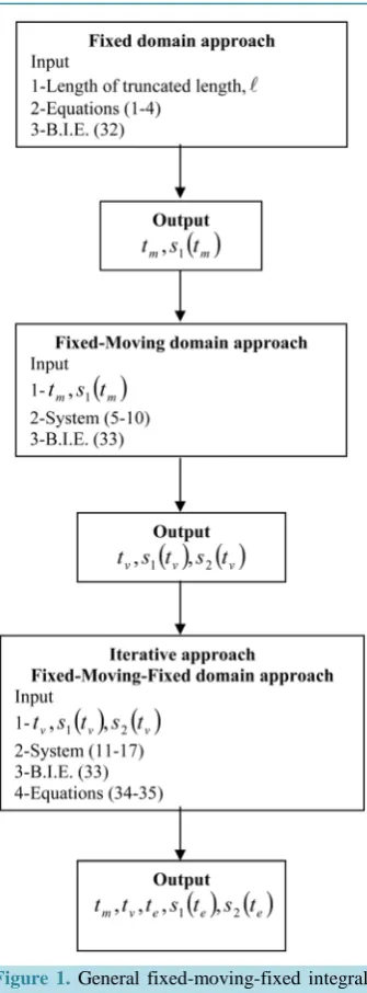
4. New Fixed-Moving-Fixed Algorithm

(5)

[image:5.595.230.398.76.530.2]

Figure 1. General fixed-moving-fixed integral

algorithm.

4.1. Algorithm and Subroutine ONEPHASE

In this subroutine, a single phase bounded by two fixed boundaries are solved, using Equation (32) and the out-put will be the time at which melting starts and the corresponding location of the first moving boundary, sepa-rating the liquid and the solid, s t₁

( )

.

Suggested Algorithm

1) Input data, mold length , spatial grid size ∆x and time step ∆t.

2) Apply the boundary integral equation, given by Equation (32) at the end points of the domain of interest to

estimate u x

(

=s t₁

( )

j ,tj

)

.

3) Check u x

(

=s t₁

( )

j ,tj

)

≥t_m,i=1, 2, ,N, if yes, then go to the next two-phase subroutine, with outputs, time of melting and the corresponding position for the moving boundary separating liquid and solid. If no update both the spatial and time variables 1

1 1 ,

j j

i i

(6)

re-quired output of this subroutine achieved.

4.2. Algorithm and Subroutine TWOPHASE

This subroutine concerns mainly with two phases each phase will be bounded by one fixed and the second is moving are solved and the output will be the time at which vapor starts and the corresponding location of the first and second moving boundaries s t₁

( )

and s₂

( )

t .

Suggested Algorithm

1) The input unit here is the output from one-phase subroutine.

2) Solve solid phase subjected to melting temperature at the moving boundary and initial temperature at the

fixed end to get

( )

1

.

t s

us x

∂

 

 _∂ 

 

3) By knowing d1

( )

d s t

t and _{( )} 1 s

s t u

x

∂

 

 _∂ 

  to estimate 1( ) . s t u

x

∂

 

 _∂ 

 



4) Check u x

(

=s t₁

( )

j ,tj

)

≥u_V, if yes, then the output of this subroutine will be the time at which vapor starts

appearing with the new position of the moving boundary separating liquid/solid and the starting position of the second moving boundary separating vapor(gas)/liquid, if no update the moving boundary separating liq-uid/solid.

4.3. Algorithm and Subroutine THREEPHASE

This subroutine is for three phases, the first one is bounded by two boundaries, one fixed and one moving, the second phase is bounded by two moving boundaries, and the third phase is also bounded by two boundaries one fixed and one moving. The output of this subroutine is to track all moving boundaries, determination all un-knowns in all phases up to the end of the process with minimum number of iterations and high prescribed accu-racy. The flow chart of this subroutine is shown in Figure 2. In this figure, the absolute errors E₁ and E₂ are defined as follow:

( )

1

( )

1

, , d

d

s

s m

u x t u x t s t

E K K L

x x ρ t

∂ ∂

 

= _ − _−

∂ ∂

 



 (34)

( )

2 2

d d v

v v

s t

u u

E K K L

x x ρ t

∂ ∂

 

= _ − _−

∂ ∂

 



 (35)

5. Numerical Results

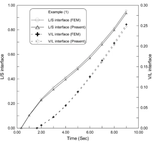
5.1. Vaporization Test Problem

In this section, three test problems are solved to check the validity of the proposed algorithm and the high accu-racy expected. The first example is a multi-moving boundary problem [13]. The thermo-physical properties are listed below in Table 1.

(7)

[image:7.595.177.487.83.437.2]

Figure 2. Flow chart for THREEPHASE subroutine.

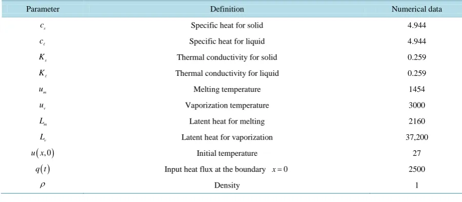
[image:7.595.183.447.461.707.2]

(8)

[image:8.595.85.536.101.298.2]

Table 1. Numerical data for vaporization test problem.

Parameter Definition Numerical data

s

c Specific heat for solid 4.944

c_ Specific heat for liquid 4.944

s

K Thermal conductivity for solid 0.259

K_ Thermal conductivity for liquid 0.259

m

u Melting temperature 1454

v

u Vaporization temperature 3000

m

L Latent heat for melting 2160

v

L Latent heat for vaporization 37,200

( )

, 0

u x Initial temperature 27

( )

q t Input heat flux at the boundary x=0 2500

ρ Density 1

Table 2. Comparison between melting, vaporization and end time.

Time step Type of time FE Present Absolute error Average number of

iterations

0.25 t

∆ =

m

t 0.36150 0.36158 5

8.0 10× −

12 - 16

v

t 1.63034 1.63041 _{7.0 10}_× −5

e

t 9.75464 9.75468 5

3.4 10× −

0.0625 t

∆ =

m

t 0.32767 0.32771 _{4.0 10}_× −5

20 - 24

v

t 1.63446 1.63449 _{3.25 10}_× −5

e

t 9.38719 9.38721 5

2.0 10× −

nearly the half.

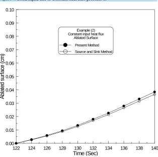
5.2. Ablation Test Problem-1

A solid medium initially at uniform temperature, ui =300 K

 _{, the boundary}_x₌₀_{exposed to two different}

cases of input heat flux, constant, Q t

( )

= ×5 106 and linear, Q t

( )

= ×3 104t respectively. The domain in the present problem is still fixed while appearing two moving interfaces, solid-liquid and vapor (gas)-liquid (Ablation surface). The results due to the present algorithm are shown in Figures 4-6, respectively and the results are com-pared with the results due to the source and sink method [14]. Figure 4 shows the movement of solid-liquid due to constant input heat flux, and the resulting ablation surface due to the same input heat flux is shown in Figure 5. The same results due to linear case are plotted on the same plot as shown in Figure 6. From the computations and figures, it is found that the solid-liquid interface has the same behavior in both constant and linear cases of input heat flux that is concave upward. In case of linear heat flux input this concavity becomes more apparent than the constant case. In the contrary, the vapor (gas)/liquid interface behaves concave downward but in linear case this concavity increases.

5.3. Ablation Test Problem-2

This problem is for a long enough solid mold initially at a uniform temperature. The surface x=0 exposed to two different high input heat flux, constant and linear and the vapor is removed as soon as it formed- ablation problem-. Two specific heat flux boundary condition are chosen in the present computations, namely,

( )

2.0,10

( )

c

q t = t t and the following values used in the calculation [15] (Table 3).

(9)

[image:9.595.156.474.85.387.2]

Figure 4. Solid/liquid due to Constant heat flux-problem-1.

Figure 5. Ablated surface due to constant heat flux-problem-1.

120 122 124 126 128 130 132 134 136 138 140

Time (Sec)

8.0 8.1 8.2 8.3 8.4 8.5 8.6 8.7 8.8 8.9 9.0 9.1 9.2 9.3 9.4 9.5 9.6 9.7 9.8 9.9 10.0

S

o

lid

/L

iq

u

id

in

te

rf

a

ce

(

cm

)

Example (2) Constant input heat flux

Solid-Liquid interface

Present Method

Source and Sink Method

122 124 126 128 130 132 134 136 138 140

Time (Sec)

0.00 0.01 0.02 0.03 0.04 0.05 0.06 0.07 0.08 0.09 0.10

A

b

la

te

d

s

u

rf

a

ce

(

cm

)

Example (2) Constant input heat flux

Ablated Surface

Present Method

[image:9.595.157.472.394.705.2]

(10)

[image:10.595.146.477.81.369.2]

Figure 6. Solid/liquid and Ablated surface due to linear heat flux-problem-1.

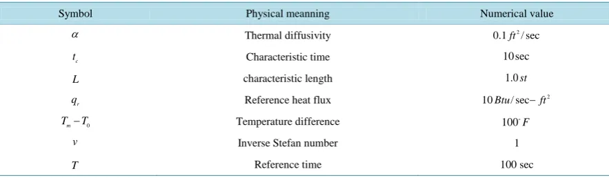
[image:10.595.145.481.386.704.2]

(11)

[image:11.595.91.533.100.229.2]

Table 3. Thermo-physical parameters.

Symbol Physical meanning Numerical value

α Thermal diffusivity 2

0.1ft / sec

c

t Characteristic time 10 sec

L characteristic length 1.0st

r

q Reference heat flux 2

10Btu/ sec−ft

0

m

T −T Temperature difference 100F

v Inverse Stefan number 1

T Reference time 100 sec

input heat flux and at the same time, the ablation thickness in case of linear heat flux is higher than that for con-stant case. There is a good agreement between the two methods in both cases.

6. Conclusion

The importance of the present paper comes from its dealing with practical applications of wide range of our dai-ly life. The boundary integral equation method is not so new but it is used as a mathematical tool due to its sim-plicity in use. Based on this method, a generalized numerical algorithm and computer code are developed to solve such applications. It is found from the computations that the developed algorithm and the code are so sim-ple to handle and that an acceptable accuracy is obtained. Also by decreasing the time step, and a little bit in-crease of iterations, the absolute errors are dein-creased to the half nearly. Finally, the algorithm and subsequently the code can be easily modified to cover higher dimensional problems with acceptable accuracy, which can be improved by decreasing the time step, but on the other hand, stability should be achieved.

References

[1] Meaad, N.M.I. (2014) Mesh-Less Methods and Its Application to Free and Moving Boundary Problems. M.Sc. Thesis, Zagazig University, Zagazig. Supervision S. G. Ahmed.

[2] Crank, J. (1984) Free and Moving Boundary Problems. Clarendon Press, Oxford.

[3] Mohamd, N.A.E. (2002) Boundary Elements Methods and Its Non-Linear Analysis of Hydrofoils. Supervisors: Prof. S. G. Ahmed and Prof. A. F. Abd-Elgawad. Zagazig University, Zagazig.

[4] Nofal, T.A. and Ahmed, S.G. (2015) An Integral Method to Solve Phase-Change Problems with/without Mushy Zones.

Journal of Applied Mathematics and Mathematics, II, 152-157.

[5] Ahmed, S.G. and Mekey, M.L. (2010) A Collocation and Cartesian Grid Methods Using New Radial Basis Function to Solve Class of Partial Differential Equations. International Journal of Computer Mathematics, 87, 1349-1362.

[6] Meshrif, S.A. and Ahmed, S.G. (2007) Approximate Integral Method Applied to Ablation Problem in a Finite Slab.

International Symposium on Recent Advances in Mathematics and Its Applications (ISRAMA 2007), Culcutta, 15-17 December 2007, 1-12.

[7] Zerroukat, M. and Chatwin, C.R. (1994) Computational Moving and Boundary Problems. Research Studies Press Ltd., Baldock.

[8] Ruan, Y. and Zabaras, N. (1991) An Inverse Finite Element Technique to Determine The change of Phase Interface Location in Two-Dimensional Melting Problem.Communications in Applied Numerical Methods, 7, 325-338.

http://dx.doi.org/10.1002/cnm.1630070411

[9] Mohamed, W.A. (2012) Advanced Mathematical Analysis for Phase Change Problems with and without Mushy Zones. Supervisors: Prof. S. G. Ahmed and Prof. M. E. Mohamed. Zagazig University, Zagazig.

[10] Liu, W., Chen, Y., Jun, S., Chen, J.-S., Belytschko, T., Pan, C., Uras, R. and Chang, C. (1996) Overview and Applica-tion of the Reproducing Kernel Particle Methods. Archive of Computational Methods in Engineering: State of the Art Reviews, 3, 3-80. http://dx.doi.org/10.1007/BF02736130

[11] Ahmed, S.G. (2005) A New Algorithm for Moving Boundary Problems Subject to Periodic Boundary Conditions. In-ternational Journal of Numerical Methods for Heat and Fluid Flow, 16, 18-27.

(12)

Wall. International Journal of Computational and Applied Mathematics, 5, 687-696.

[13] Ahmed, S.G. (2003) A New Algorithm for Front Tracking of Ablation Problem in Unbounded Domain. Ain Shams University, Egypt.

[14] Mehdi, A. and Hsieh, C.K. (1994) Solution of Ablation and Combination of Ablation and Stefan Problems by a Source and Sink Method. Numerical Heat Transfer, Part A, 26, 67-86. http://dx.doi.org/10.1080/10407789408955981

[15] Ahmed, S.G. (2003) A Numerical Solution for Nonlinear Heat Flow Problem Using Boundary Integral Method. 6th International Conference of Computer Methods and Experimental Measurements for Surface Treatment, Crete, March 2003.