UNSTEADY MHD OSCILLATORY FLOW OF JEFFREY FLUID, HEAT AND MASS TRANSFER BETWEEN PARALLEL PLATES WITH CHEMICAL REACTION AND HEAT SOURCE

(1)

UNSTEADY MHD OSCILLATORY FLOW OF JEFFREY FLUID, HEAT

AND MASS TRANSFER BETWEEN PARALLEL PLATES WITH

CHEMICAL REACTION AND HEAT SOURCE

P.R. Sharma1 and Tripti Mehta2

1,2

Department of Mathematics, University of Rajasthan, Jaipur-302004 (Raj.), India.

ABSTRACT

Aim of the paper is to investigate the effect of heat and mass transfer on unsteady MHD oscillatory flow of Jeffrey fluid between parallel plates with chemical reaction and heat source. One plate is moving and temperature prescribed at both plates is uniform and asymmetric. The effect of heat transfer on unsteady MHD oscillatory flow of fluid in vertical media are encountered in a wide range of engineering and industrial applications such as molten iron flow, recovery extraction of crude oil, geothermal systems. Numerical results for the velocity, temperature and concentration profiles for various physical parameters as well as the local skin friction coefficient, local Nusselt number and Sherwood number are discussed and presented graphically.

Keywords:

Jeffrey fluid, MHD, oscillatory flow, heat and mass transfer, chemical reaction, heat source.

1. Introduction

Oscillatory flow has known to result in higher rates of heat and mass transfer. Many

studies have been done to understand its characteristics in different systems such as

reciprocating engines, pulse combusters and chemical reactors. The chemical reaction effects

are considered in many applications of heat and mass transfer especially those encountered in

chemical reactors of porous structure, geothermal reservoirs, enhanced oil recovery etc.

Researchers have considerable interest in the study of flow between two parallel plates.

Because of its occurrence in rheometric experiments to determine the constitutive properties

(2)

Bejan and Khair (1985) obtained heat and mass transfer by natural convection in a

porous medium. Deka, Das and Soundalgekar (1994) studied the effect of mass transfer on

flow past an impulsively started infinite vertical plate with constant heat flux and chemical

reaction. Sharma and Sharma (1997) discussed unsteady flow and heat transfer between two

parallel plates. Sharma and Kumar (1998) analyzed unsteady flow and heat transfer between

two horizontal plates in the presence of transverse magnetic field. Acharya, Dash and Singh

(2000) discussed magnetic field effects on the free convection and mass transfer flow through

porous medium with constant suction and constant heat flux. Kim (2000) explained unsteady

MHD convective heat transfer past a semi infinite vertical porous moving plate with variable

suction. Chamkha (2003) presented MHD flow of a numerical of uniformly stretched vertical

permeable surface in the presence of heat generation/absorption and chemical reaction.

Sharma and Chaturvedi (2003) described unsteady flow and heat transfer of an electrically

conducting viscous incompressible fluid between two non-conducting parallel porous plates

under uniform transverse magnetic field.

Sharma, Chawla and Singh (2005) discussed unsteady plane Poiseuille flow and heat

transfer in the presence of oscillatory temperature of the lower plate. Makinde and Mhone

(2005) presented heat transfer to MHD oscillatory flow in a channel filled with porous

medium. Sharma and Singh (2008) derived effects of variable thermal conductivity and heat

source/sink on MHD flow near a stagnation point on a linearly stretching sheet. Pal and

Talukdar (2010) obtained unsteady magnetohydrodynamic convective heat and mass transfer

in a boundary layer slip flow past a vertical permeable plate with thermal radiation and

chemical reaction. Israel-Cookey and Nwaigwe (2010) studied unsteady MHD flow of a

radiating fluid over a moving heated porous plate with time-dependent suction. Bakr (2011)

described effects of chemical reaction on MHD free convection and mass transfer flow of a

micropolar fluid with oscillatory plate velocity and constant heat source in a rotating frame of

reference. Shateyi and Motsa (2011) considered unsteady magnetohydrodynamic convective

heat and mass transfer past an infinite vertical plate in a porous medium with thermal

radiation heat generation/absorption and chemical reaction.

Kavita, Prasad and Kumari (2012) discussed slip effects on MHD oscillatory flow of

Jeffrey fluid in a channel with heat transfer. Kumar, Jain and Gupta (2012) presented

unsteady MHD free convection flow through porous medium sandwiched between viscous

(3)

oscillatory flow of Jeffrey fluid in a channel. Sreenadh, Devaki and Diwakar (2012) studied

unsteady flow of Jeffrey fluid in an elastic tube with steno sis. Vineet, Gupta and Varshney

(2012) considered MHD effects on free convection fluid flow past a vertical surface with

porous medium and radiation. Asadullah, Umar, Nareed, Raheela and Mohyuddin (2013)

discussed MHD flow of a Jeffrey fluid in converging and diverging channels. Devika, Satya

Narayana and Venkataramana (2013) presented MHD oscillatory flow of a visco elastic fluid

in a porous channel with chemical reaction.

Aim of the paper is to investigate effects of heat and mass transfer on unsteady MHD

oscillatory flow of Jeffrey fluid between parallel plates with chemical reaction and heat

source. Equations of momentum, energy and diffusion, which govern the fluid flow, heat and

mass transfer are solved by using perturbation method. The effects of various physical

parameters on fluid velocity, temperature, concentration, skin friction coefficient, Nusselt

number and Sherwood number at the plates are derived, discussed numerically and shown

through graphs.

2. Mathematical analysis:

Consider an oscillatory flow of Jeffrey fluid and heat transfer through a vertical

infinite channel with chemical reaction and heat source with one moving plate in the presence

of transverse magnetic field. The channel width is

d

. Following Kavita et al., that the constitute equation of S for Jeffrey fluid is given by

















₂

* 2 2 * 1

1

dt

d

dt

d

S











,

...(1)

where



the dynamic viscosity,



₁ the ratio of relaxation to retardation times,



₂ the

retardation time, _*

dt

d



the shear rate and

t

* the time.

The radiative heat term in horizontal direction is considered negligible in comparison with

(4)

temperatures of the plates. The

x

*-axis is taken along the plate (when y0) and a straight

line perpendicular to that as the

y

*-axis. A magnetic field of uniform strength

B

₀ is applied

normal to the plate along

x

*-direction and the induced magnetic field is assumed negligible. It is also assumed that the fluid has small electrical conductivity and the electromagnetic

force produced is very small. The pressure gradient is also assumed negligible. Since the

plate is considered infinite in

x

*-direction, all the physical variables will be independent of

*

x

and are functions of

y

*and

t

*. Under the usual Boussinesq’s approximation, the

governing equations of motion, energy and mass conservation are given by





T



w



C



w



e

C

g

T

g

u

B

y

u

x

P

t

u























* * * 2 0 2 * * 2 1 * * * *

1













, ...(2)



w



p

Q

T

y

q

y

T

t

T

C















* * 2 * * 2 * *





, ...(3)



w



C

K

y

C

D

t

C









* 2 * * 2 * * , …(4)

where

u

*denotes fluid velocity along

x

*-axis,

t

*the time,

P

*fluid pressure,

T

*fluid temperature,

C

*concentration of fluid,



the dynamic viscosity,



_{fluid density,}



₁ the ratio of relaxation to retardation times,



₂ the retardation time,



_e electric conductivity,

g

acceleration due to gravity,



_T coefficient of the thermal expansion,



_C coefficient of mass expansion,



thermal conductivity,

C

_p specific heat at constant pressure,

q

radiative heat

flux in the

y

*-direction,

Q

heat generation/ absorption constant,

D

the mass diffusion coefficient and

K

_C the chemical reaction coefficient.

The boundary conditions are given by



,



0

,



,



,



,



;

:

0

* * * * * * * * *

*

w

C

y

t

C

T

t

y

T

t

y

u

y





,





1

 

,









1



,

:

* * * * *

* i t

w w t i *

e

T

t

y

T

e

U

t

y

u

d

(5)











i t



w

C

e

C

t

y

C

* *

,

*





_



1







.

…(5)

Following Cogley et al. (1968), that the fluid is optically thin with a relative low density and radiative heat flux is given by



*



2

*

4

T

y

q

w









. …(6)

Introducing the following dimensionless quantities

d

x

*



,

d

y

*



, 



U

u

* , w w

T





 *



, w w

C





 * ,

d

U

t





*

,





U

_

d



Re

,





2 2

0

2

B

d

Ha



e

,





dU

C

_p

Pe



 ,





2 2 2

4

d

N



,





U

d

K

J

C ,

D

dU

Sc



 ,



2

Qd

S



,





 





U

T

g

d

Gr

T w







2 ,





 





U

C

g

d

Gc

C w







2

;

…(7)

into the equations (2), (3), (4), we get





y

Ha

u

Gr

GcC

u

t

u

















2 2 2 1

1

Re

, …(8)



S

N

y

t

Pe









2 2 2 , …(9)

JC

y

C

Sc

t

C









2 2

1

, …(10)

where

u

is dimensionless velocity,

t

the dimensionless time,

y

dimensionless coordinate

(6)

number,

Pe

Peclet number,

N

Radiation parameter,

S

heat source parameter,

Sc

Schmidt

number and

J

chemical reaction parameter.

The dimensionless boundary conditions are given by

 

,

0

,

 

,

0

,

 

,

0

:

0



u

y

t

y

t

C

y

t

y



;

 

i t

 

i t

 

i t

e

t

y

C

e

t

y

e

t

y

u

y



1

:

,



1







,



,



1







,



1





 .

…(11)

3. Method of Solution

In order to solve equations (8), (9) and (10) under the boundary conditions (11) assuming

 

2

1 0

,

t

u

y



u

y

e



O



y

u





i t



,

 

2

1 0

,











O

e

y

t

y





i t



,

 

2

1 0

,

t

C

y



C

y

e



O



y

C





i t



,

...(12)

using (12) into the equations (8), (9) and (10), equating the coefficients of the harmonic and non-harmonic terms and neglecting the coefficients of



2, we obtain

 

y

Ha

u

 

y

Gr

 

y

GcC

 

y

u

a

2 ₀ ₀ ₀

0 2

1

''











,

...(13)

 

y

b

u

 

y

Gr

 

y

GcC

 

y

u

a

₁2 ₁

''



₁2 ₁







₁



₁ ,

...(14)

 

0

''

0

2 2

0

y



a



y





,

...(15)

 

0

''

₂2 ₁

1

y



b



y





,

...(16)

 

0

''

0

2 3

0

y



a

C

y



C

,

...(17)

 

0

''

1

2 3

1

y



b

C

y



C

.

(7)

where 1 2 1

1







a

, 2 2

Re

1

Ha

i



b





,

a

2



N

2



S

2 ,

b



N



S



i



Pe

2

2 ,

Sc

K

a

32



and

b



K

Sc



i



Sc

2

3 .

Now, the corresponding boundary conditions are reduced to

 

0

,

 

0

,

 

0

:

0

₀



₀



₀



u

y

C

y



;

u

₁

 

y



0

,



₁

 

y



0

,

C

₁

 

y



0

;

 

1

,

 

1

,

 

1

:

1

₀



₀



₀



u

y

C

y



;

u

₁

 

y



1

,



₁

 

y



1

,

C

₁

 

y



1

.

…(19)

Equations (13) to (18) are ordinary second order differential equations and solved under the

boundary conditions (19). Through straight forward calculations

u

₀

 

y

,

u

₁

 

y

,



₀

 

y

,

 

y

1



, C₀

 

y and

C

₁

 

y

are known. Finally, the expressions of u

 

y,t ,



 

y,t and C

 

y,t

are known as given below

 



 



































2 2 2 2 2 2 1 1 1 2 2 3 2 1 2 2 2 2 1

sin

sinh

1

,

a

y

a

Ha

a

Gr

p

y

p

Ha

a

Gc

Ha

a

Gr

t

y

u











 

































1 1 2 1 2 3 2 1 2 1 2 2 2 1 3 3 2 2 3 2 1

sinh

1

sinh

q

y

q

b

a

Gc

b

a

Gr

a

y

a

Ha

a

Gc











i t

e

b

y

b

a

Gc

b

y

b

a

Gr













3 3 2 1 2 3 2 1 2 2 2 1 2 2 2 1

sinh

sin

, ...(20)

 

i t

e

b

y

b

a

y

a

t

y







2 2 2 2

sin

,





, ...(21)

 

i t

e

b

y

b

a

y

a

t

y

C





3 3 3 3

sinh

,





, ...(22)

(8)

dy

du

e

dy

du

dy

du

C

i t

f

1 0









at

y



0

and

y



1

,

…(23)

Hence, skin-friction coefficient at the plate (when

y



0

) is given by

 



 



































2 2 2 2 2 2 1 1 1 2 2 3 2 1 2 2 2 2 1 0

sin

sinh

1

a

Ha

a

Gr

p

Ha

a

Gc

Ha

a

Gr

C

f











 

































1 1 2 1 2 3 2 1 2 1 2 2 2 1 3 3 2 2 3 2 1

sinh

1

sinh

q

b

a

Gc

b

a

Gr

a

Ha

a

Gc











i t

e

b

a

Gc

b

a

Gr













3 3 2 1 2 3 2 1 2 2 2 1 2 2 2

1

sin

sinh

,

...(24)

The skin-friction coefficient at the plate (wheny 1) is given by

 



 



































2 2 2 2 2 2 2 1 1 1 1 2 2 3 2 1 2 2 2 2 1 1

sin

cos

sinh

cosh

1

a

Ha

a

Gr

p

Ha

a

Gc

Ha

a

Gr

C

f











 

































1 1 1 2 1 2 3 2 1 2 1 2 2 2 1 3 3 3 2 2 3 2 1

sinh

cosh

1

sinh

cosh

q

b

a

Gc

b

a

Gr

a

Ha

a

Gc











i t

e

b

a

Gc

b

a

Gr













3 3 3 2 1 2 3 2 1 2 2 2 2 1 2 2 2 1

sinh

cosh

sin

cos

. ...(25)

The dimensionless rate of heat transfer in terms of the Nusselt number at both the plates is given by





































dy

d

e

dy

d

y

Nu



0



it



1

at

y



0

and

y



1

,

...(26)

(9)

 

i t

e

b

a

Nu





2 2 2

2 0

sin





,

…(27)

The Nusselt number at the plate (wheny1) is given by

 

i t

e

b

a

Nu





2 2 2

1

sin

cos

sin

cos





.

…(28)

The dimensionless rate of mass transfer in terms of the Sherwood number at both the plates is given by



















y

C

Sh

at

y



0

and

y



1

,

…(29)

Hence, the Sherwood number at the plate (when

y



0

) is given by

 

i t

e

b

a

Sh





3 3 3

3 0

sinh





,

…(30)

The Sherwood number at the plate (wheny1) is given by

 

i t

e

b

a

Sh





3 3 3

1

sinh

cosh

sinh

cosh





.

…(31)

4. Results and Discussions

It is observed from figure 1 that as Grashof number increases, the velocity increases.

Therefore, for higher values of Grashof number the flow at the boundary is turbulent while

for lower values the flow at the boundary is laminar.

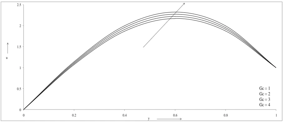
Figure 2 shows that with the increase in modified Grashof number contributes to the

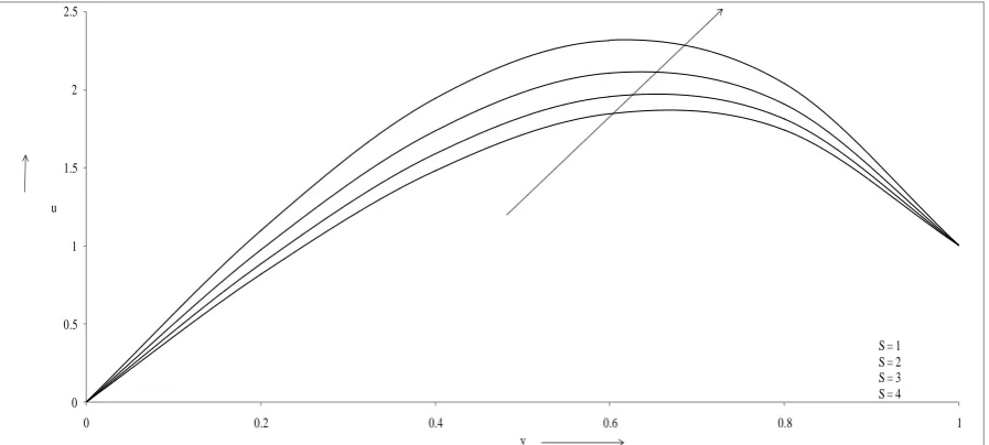
rise in velocity of the fluid. Figure 3 illustrates that the velocity of the fluid decreases as the

values of Hartmann number increases. Figure 4 reveals that velocity increases as heat source

(10)

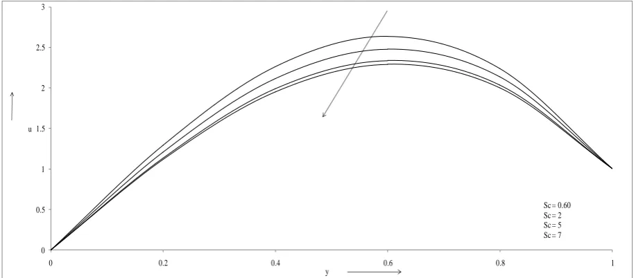
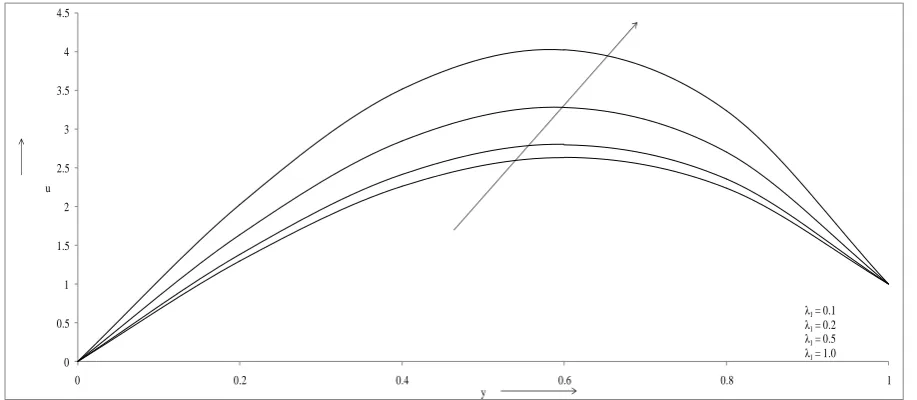
increase in chemical reaction parameter results in decreasing the fluid velocity. Figure 8

demonstrates that the velocity increases with increase in material parameter. The ratio of

relaxation to retardation times enhances the increase flow of velocity when it becomes large.

Figure 9 shows that the increase in the heat source parameter significantly increase the

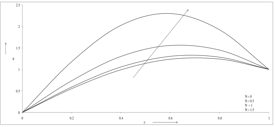
thermal buoyancy effects which rise fluid temperature. Figure 10 illustrates that increase in

the radiation parameter increases the fluid temperature because of large values of radiation

parameter oppose the conduction over radiation, thereby which increases the buoyancy force

and increases the thickness of the thermal boundary layer.

Figure 11 represents that an increase in Schmidt number results in decreasing the fluid

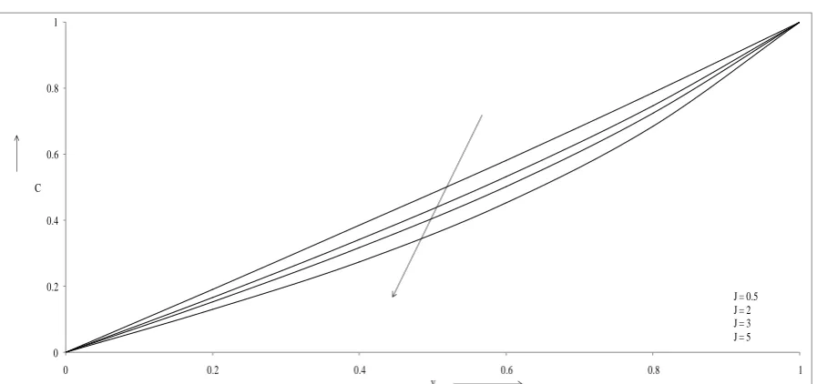
concentration. Figure 12 shows concentration decreases for increasing the chemical reaction

parameter which indicates that the diffusion rates can be tremendously changed by the

chemical reaction.

It is seen from Table 1 and Table 2 that the velocity decreases with the increase in

Reynolds number and Peclet number. Table 3 shows that the velocity of the fluid is inversely

proportional to the frequency of the oscillation, thus increasing of frequency reduces the

velocity of the fluid. It is observed from Table 4 and Table 5 that the fluid temperature

decreases with increase in Peclet number and frequency of oscillation. It is noted from Table

6 that the concentration of the fluid decreases with an increase in frequency of the oscillation.

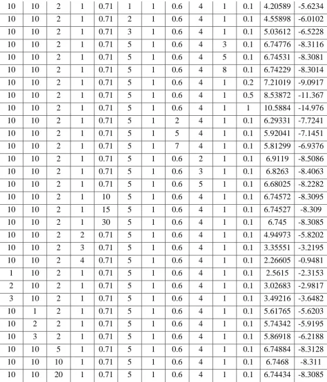
It is observed from Table 7 that the skin friction coefficient at the plate (when y0)

increases due to increase in Grashof number, modified Grashof number, heat source

parameter, radiation parameter or material parameter, while it decreases due to increase in

Reynolds number, Hartmann number, Peclet number, Schmidt number, chemical reaction

parameter or frequency of the oscillation. The skin-friction coefficient at the plate (when

1 

y ) increases due to increase of Reynolds number, Hartmann number, Peclet number,

Schmidt number, chemical reaction parameter or frequency of the oscillation, while it

decreases due to increase of Grashof number, modified Grashof number, heat source

parameter, radiation parameter or material parameter.

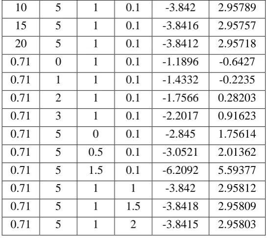
It is noted from Table 8 that the Nusselt number at the plate (when y0) increases

due to increase in Peclet number or frequency of the oscillation, while it decreases due to

increase in heat source parameter or radiation parameter, but opposite behaviour is seen at the

(11)

It is seen from Table 9 that the Sherwood number at the plate (when y0) increases

due to increase in Schmidt number, chemical reaction parameter or frequency of the

oscillation. The Sherwood number at the plate (when y1) increases due to increase in

frequency of the oscillation, while it decreases due to increase of Schmidt number or

chemical reaction parameter.

0 0.2 0.4 0.6 0.8 1 1.2 1.4 1.6 1.8

0 0.2 0.4 0.6 0.8 1

u

y

[image:11.595.72.523.234.426.2]

Gr = 1 Gr = 2 Gr = 3 Gr = 4

Figure 1. Velocity profiles versus

y

for different values of GrwhenGc=10, Re=2, Ha=1.0, Pe=0.71, S=5.0, N=1.0, Sc=0.60, J=0.5, ω=0.1, ε=0.001, t=0.5, λ1=0.1.

0 0.5 1 1.5 2 2.5

0 0.2 0.4 0.6 0.8 1

u

y

Gc = 1 Gc = 2 Gc = 3 Gc = 4

[image:11.595.72.525.473.669.2]

(12)

0 0.5 1 1.5 2 2.5 3

0 0.2 0.4 0.6 0.8 1

u

y

[image:12.595.75.531.77.297.2]

Ha = 1 Ha = 2 Ha = 3 Ha = 4

y

for different values of

Ha

whenGr=10, Gc=10, Re=2, Pe=0.71, S=5.0, N=1.0, Sc=0.60, J=0.5, ω=0.1, ε=0.001, t=0.5, λ1=0.1.

0 0.5 1 1.5 2 2.5

0 0.2 0.4 0.6 0.8 1

u

y

S = 1 S = 2 S = 3 S = 4

[image:12.595.74.523.351.553.2]

(13)

0 0.5 1 1.5 2 2.5 3 3.5

0 0.2 0.4 0.6 0.8 1

u

y

N = 0 N = 0.5 N = 1 N = 1.5

y

N

whenGr=10, Gc=10, Re=2, Ha=1.0, Pe=0.71, S=5.0, Sc=0.60, J=0.5, ω=0.1, ε=0.001, t=0.5, λ1=0.1.

0 0.5 1 1.5 2 2.5 3

0 0.2 0.4 0.6 0.8 1

u

y

[image:13.595.74.524.76.289.2]

Sc = 0.60 Sc = 2 Sc = 5 Sc = 7

[image:13.595.72.531.343.544.2]

(14)

0 0.5 1 1.5 2 2.5 3

0 0.2 0.4 0.6 0.8 1

u

y

J = 0.50 J = 2.0 J = 3.0 J = 5.0

y

J

when Gr=10, Gc=10, Re=2, Ha=1.0, Pe=0.71, S=5.0, N=1.0, Sc=0.60, ω=0.1, ε=0.001, t=0.5, λ1=0.1.

0 0.5 1 1.5 2 2.5 3 3.5 4 4.5

0 0.2 0.4 0.6 0.8 1

u

y

λ1= 0.1

λ1= 0.2

λ1= 0.5

λ1= 1.0

[image:14.595.71.531.76.300.2] [image:14.595.71.530.350.550.2]

(15)

0 0.2 0.4 0.6 0.8 1 1.2 1.4

0 0.2 0.4 0.6 0.8 1

θ

y

S = 1 S = 2 S = 3 S = 4

Figure 9. Temperature profiles versus

y

S

when Gr=10, Gc=10, Re=2, Ha=1.0, Pe=0.71, N=1.0, Sc=0.60, J=0.5, ω=0.1, ε=0.001, t=0.5, λ1=0.1.

0 0.5 1 1.5 2 2.5

0 0.2 0.4 0.6 0.8 1

θ

y

N = 0 N = 0.5 N = 1 N = 1.5

[image:15.595.73.530.73.299.2] [image:15.595.73.528.346.556.2]

(16)

0 0.2 0.4 0.6 0.8 1

C

y

[image:16.595.74.524.72.290.2]

Sc = 0.6 Sc = 2 Sc = 5 Sc = 7

Figure 11. Concentration profiles versus

y

Sc

whenGr=10, Gc=10, Re=2, Ha=1.0, Pe=0.71, S=5.0, N=1.0, J=0.5, ω=0.1, ε=0.001, t=0.5, λ1=0.1.

0 0.2 0.4 0.6 0.8 1

C

y

J = 0.5 J = 2 J = 3 J = 5

Figure 12. Concentration profiles versus

y

J

when Gr=10, Gc=10, Re=2, Ha=1.0, Pe=0.71, S=5.0, N=1.0, Sc=0.60, ω=0.1, ε=0.001, t=0.5, λ1=0.1.

Table 1. Velocity profiles with

y

for different

values of

Re

when Gr=10, Gc=10, Ha=1.0,

Pe=0.71, S=5.0, N=1.0, Sc=0.60, J=4, ω=1, ε=0.001, t=0.5, λ1=0.1.

y Re=1 Re=5 Re=10 Re=20

0 0 0 0 0

0.2 1.2938

2

1.2937 1

1.2933 2

1.2928 6

0.4 2.2628 2.2627 2.2620 2.2613

0.6 2.6372 2.6370

4

2.6364 3

2.6356

0.8 2.2405

1

2.2404 3

2.2400 6

2.2395 4

1 1.0008

8

1.0008 8

Table 2. Velocity profiles with

y

for different

values of

Pe

when Gr=10, Gc=10, Re=2, [image:16.595.77.526.334.545.2]

(17)

y Pe=0.71 Pe=10 Pe=15 Pe=30

0 0 0 0 0

0.2 1.29383 1.29312 1.29304 1.29298

0.4 2.2629 2.26176 2.26162 2.26151

0.6 2.63723 2.63609 2.63594 2.63581

0.8 2.24053 2.23983 2.23974 2.23964

1 1.00088 1.00088 1.00088 1.00088

Table 3. Velocity profiles versus

y

for different

values of



whenGr=10, Gc=10, Re=2, Ha=1.0,

Pe=0.71, S=5.0, N=1.0, Sc=0.60, J=4, ε=0.001, t=0.5, λ1=0.1.

y ω=1 ω=3 ω=5 ω=8

0 0 0 0 0

0.2 1.2938

3 1.2934 9 1.2930 1 1.2924 2

0.4 2.2629 2.2622

5

2.2613 5

2.2603 2

0.6 2.6372

3 2.6363 5 2.6351 6 2.6339 7

0.8 2.2405

3 2.2395 7 2.2383 2 2.2374 6

1 1.0008

8

1.0000 7

0.9992 0.9993

5

Table 4. Temperature profiles versus

y

for

different values of

Pe

when Gr=10, Gc=10,

Re=2, Ha=1.0, S=5.0, N=1.0, Sc=0.60, J=4, ω=1, ε=0.001, t=0.5, λ1=0.1.

y Pe=0.7

1

Pe=10 Pe=15 Pe=30

0 0 0 0 0

0.2 0.7380

3

0.7373 9

0.7373 0.7372

8

0.4 1.3024

5 1.3014 2 1.3012 6 1.3011 6

0.6 1.5604

7 1.5594 5 1.5592 8 1.5590 9

0.8 1.4513

9 1.4507 9 1.4506 8 1.4505 2

1 1.0008

8 1.0008 8 1.0008 8 1.0008 8

Table 5. Temperature profiles versus

y

for

different values of



when Gr=10, Gc=10,

Re=2, Ha=1.0, Pe=0.71, S=5.0, N=1.0, Sc=0.60, J=4, ε=0.001, t=0.5, λ1=0.1.

y ω=1 ω=3 ω=5 ω=8

0 0 0 0 0

0.2 0.7380

3 0.7377 6 0.7373 6 0.7369 7

0.4 1.3024

5 1.3019 2 1.3011 9 1.3005 4

0.6 1.5604

7

1.5597 5

1.5588 1.5581

2

0.8 1.4513

9 1.4505 8 1.4495 6 1.4491 5

1 1.0008

8

1.0000 7

0.9992 0.9993

5

Table 6. Concentration profiles versus

y

for

different values of



when Gr=10, Gc=10,

Re=2, Ha=1.0, Pe=0.71, S=5.0, N=1.0, Sc=0.60, J=4.0, ε=0.001, t=0.5, λ1=0.1.

y ω=1 ω=3 ω=5 ω=8

0 0 0 0 0

0.2 0.1402 0.14011 0.14 0.13994

0.4 0.29396 0.29377 0.29353 0.29343

0.6 0.47616 0.47584 0.47545 0.47533

0.8 0.70444 0.70392 0.70332 0.70327

1 1.00088 1.00007 0.9992 0.99935

Table 7. Numerical values of skin friction coefficient at the plates for different values of physical parameters

Gr Gc Re Ha Pe S N Sc J ω λ1 τ0 τ1

10 10 2 1 0.71 5 1 0.6 4 1 0.1 6.7495 -8.3132

10 10 2 1 0.71 5 0 0.6 4 1 0.1 5.71417 -7.2383

(18)

10 10 2 1 0.71 1 1 0.6 4 1 0.1 4.20589 -5.6234

10 10 2 1 0.71 2 1 0.6 4 1 0.1 4.55898 -6.0102

10 10 2 1 0.71 3 1 0.6 4 1 0.1 5.03612 -6.5228

10 10 2 1 0.71 5 1 0.6 4 3 0.1 6.74776 -8.3116

10 10 2 1 0.71 5 1 0.6 4 5 0.1 6.74531 -8.3081

10 10 2 1 0.71 5 1 0.6 4 8 0.1 6.74229 -8.3014

10 10 2 1 0.71 5 1 0.6 4 1 0.2 7.21019 -9.0917

10 10 2 1 0.71 5 1 0.6 4 1 0.5 8.53872 -11.367

10 10 2 1 0.71 5 1 0.6 4 1 1 10.5884 -14.976

10 10 2 1 0.71 5 1 2 4 1 0.1 6.29331 -7.7241

10 10 2 1 0.71 5 1 5 4 1 0.1 5.92041 -7.1451

10 10 2 1 0.71 5 1 7 4 1 0.1 5.81299 -6.9376

10 10 2 1 0.71 5 1 0.6 2 1 0.1 6.9119 -8.5086

10 10 2 1 0.71 5 1 0.6 3 1 0.1 6.8263 -8.4063

10 10 2 1 0.71 5 1 0.6 5 1 0.1 6.68025 -8.2282

10 10 2 1 10 5 1 0.6 4 1 0.1 6.74572 -8.3095

10 10 2 1 15 5 1 0.6 4 1 0.1 6.74527 -8.309

10 10 2 1 30 5 1 0.6 4 1 0.1 6.745 -8.3085

10 10 2 2 0.71 5 1 0.6 4 1 0.1 4.94973 -5.8202

10 10 2 3 0.71 5 1 0.6 4 1 0.1 3.35551 -3.2195

10 10 2 4 0.71 5 1 0.6 4 1 0.1 2.26605 -0.9481

1 10 2 1 0.71 5 1 0.6 4 1 0.1 2.5615 -2.3153

2 10 2 1 0.71 5 1 0.6 4 1 0.1 3.02683 -2.9817

3 10 2 1 0.71 5 1 0.6 4 1 0.1 3.49216 -3.6482

10 1 2 1 0.71 5 1 0.6 4 1 0.1 5.61765 -5.6203

10 2 2 1 0.71 5 1 0.6 4 1 0.1 5.74342 -5.9195

10 3 2 1 0.71 5 1 0.6 4 1 0.1 5.86918 -6.2188

10 10 5 1 0.71 5 1 0.6 4 1 0.1 6.74884 -8.3128

10 10 10 1 0.71 5 1 0.6 4 1 0.1 6.7468 -8.311

[image:18.595.72.547.86.641.2]

10 10 20 1 0.71 5 1 0.6 4 1 0.1 6.74434 -8.3085

Table 8. Numerical values of Nusselt number at the plates for different values of physical parameters

Pe S N ω Nu0 Nu1

(19)

10 5 1 0.1 -3.842 2.95789

15 5 1 0.1 -3.8416 2.95757

20 5 1 0.1 -3.8412 2.95718

0.71 0 1 0.1 -1.1896 -0.6427

0.71 1 1 0.1 -1.4332 -0.2235

0.71 2 1 0.1 -1.7566 0.28203

0.71 3 1 0.1 -2.2017 0.91623

0.71 5 0 0.1 -2.845 1.75614

0.71 5 0.5 0.1 -3.0521 2.01362

0.71 5 1.5 0.1 -6.2092 5.59377

0.71 5 1 1 -3.842 2.95812

0.71 5 1 1.5 -3.8418 2.95809

[image:19.595.161.435.88.331.2]

0.71 5 1 2 -3.8415 2.95803

Table 9. Numerical values of Sherwood number at the plates for different values of physical parameters

Sc J ω Sh0 Sh1

0.6 4 1 -0.6899 -1.697

0.6 4 3 -0.6895 -1.6953

0.6 4 5 -0.6889 -1.6937

2 4 1 -0.3358 -2.8506

5 4 1 -0.1023 -4.477

7 4 1 -0.0533 -5.2961

0.6 2 1 -0.8256 -1.3724

0.6 3 1 -0.7536 -1.5397

0.6 5 1 -0.6333 -1.8455

5. Conclusions:

Effect of heat and mass transfer on unsteady MHD oscillatory flow of Jeffrey fluid between

parallel plates in the presence of chemical reaction and heat source is investigated. The

velocity, temperature and concentration profiles are obtained and shown through graphs,

dimensionless shear stress, rate of heat and mass transfer at the plates are derived and their

numerical values are presented through tables. In view of the above, the following conlusions

(20)

(i) The velocity and temperature of the fluid increases as the heat source parameter or

radiation parameter.

(ii) The velocity and temperature of the fluid decrease with the increase of Peclet number

or frequency of the oscillation.

(iii) Due to increase in Schmidt number, chemical reaction parameter or frequency of the

oscillation, the velocity and concentration of the fluid decrease.

(iv) As Grashof number, modified Grashof number, heat source parameter, radiation

parameter or material parameter increases the skin-friction coefficient increases at the

plate (when y0) while decreases at the plate (when y1).

(v) An increase in Reynolds number, Hartmann number, Peclet number or Schmidt

number causes an increase in skin-friction coefficient at the plate (when y1), while

it decreases at the plate (when y0).

(vi) The rate of heat transfer at the plate (when y0) increases due to increase in Peclet

number or frequency of the oscillation, while it decreases as the heat source parameter

or radiation parameter increases.

(vii) The rate of heat transfer at the plate (when y1) increases due to increase in heat

source parameter or radiation parameter while it decreases due to increase in Peclet

number or frequency of the oscillation.

(viii) Due to increase in frequency of the oscillation, the rate of mass transfer increases at

both the plates.

(ix) An increase in Schmidt number or chemical reaction parameter leads to an increase in

the rate of mass transfer at the plate (when y0), while it decreases at the plate

(when y1).

6. References:

1. Acharya, M; Dash, G. C. and Singh, L. P., “Magnetic field effects on the free convection and mass transfer flow through porous medium with constant suction and constant heat flux”. Indian J. Pure Appl. Math., Vol. 31, 2000, pp. 1-8.

(21)

3. Bakr, A. A., “Effects of chemical reaction on MHD free convection and mass transfer flow of a micropolar fluid with oscillatory plate velocity and constant heat source in a rotating frame of reference”. Comm. Nonlinear Sci. Num. Simulat., Vol. 16, 2011, pp. 698-710.

4. Bejan, A. And Khair, K. R., “ Heat and mass transfer by natural vonvection in a porous medium”. Int. J. Heat Mass Transfer, Vol. 28, 1985, pp. 909-918.

5. Chamkha, A. J., “MHD flow of a numerical of uniformly stretched vertical permeable

surface in the presence of heat generation/absorption and chemical reaction”. Int. Comm. Heat Mass transfer, Vol. 30, 2003, pp. 413-422.

6. Deka, R.; Das, U. N. and Soundalgekar, V. M., “Effect of mass transfer on flow past

an impulsively started infinite vertical plate with constant heat flux and chemical reaction”. Forschung Ingenieurwesen, Vol.60, 1994, pp. 284-287.

7. Devika, B.; Satya Narayana, P. V. And Venkataramana, S., “MHD oscillatory flow of

a visco elastic fluid in a porous channel with chemical reaction”. Int. J. of Engg. Sci. Invention, Vol. 2, 2013, pp. 26-35.

8. Israel-Cookey, C. and Nwaigwe, C., “Unsteady MHD flow of a radiating fluid over a

moving heated porous plate with time-dependent suction”. Am. J. Sci. Ind. Res., Vol. 1, 2010, pp. 88-95.

9. Kavita, K.; Prasad, R. K. and Kumari, B. A., “Slip effects on MHD oscillatory flow of

Jeffrey fluid in a channel with heat transfer”. Int. J. Math. Arch., Vol. 3, 2012, pp. 2903-2911.

10. Kavita, K.; Prasad, R. K. and Kumari, B. A., “Influence of heat transfer on MHD oscillatory flow of Jeffrey fluid in a channel”. Adv. Appl. Sci. Res., Vol. 3, 2012, pp. 2312-2325.

11. Kim, U. J., “Unsteady MHD convective heat transfer past a semi infinite vertical porous moving plate with variable suction”. Int. J. Eng. Sci. Vol. 38, 2000, pp. 833-845.

12. Kumar, N; Jain, T. and Gupta, S., “Unsteady MHD free convection flow through porous medium sandwiched between viscous fluids”. Int. J. Ener. Tech., Vol. 4, 2012, pp. 1-11.

13. Makinde, O. D. and Mhone, P. Y., “Heat transfer to MHD oscillatory flow in a channel filled with porous medium”. Romanian J. Physics, Vol. 50, 2005, pp. 931-938.

14. Pal, D. and Talukdar, B., “Perturbation analysis of unsteady magnetohydrodynamic convective heat and mass transfer in a boundary layer slip flow past a vertical permeable plate with thermal radiation and chemical reaction”. Communications in Nonlinear Science and Numerical Simulation, Vol. 15, 2010, pp. 1813-1830.

15. Sharma, P. R. and Singh, G., “Effects of variable thermal conductivity and heat source/sink on MHD flow near a stagnation point on a linearly stretching sheet”. J. of appl. fluid mechanics, Vol. 2, 2008, pp. 13-22.

(22)

17. Sharma, P.R. and Kumar, N., “Unsteady flow and heat transfer between two horizontal plates in the presence of transverse magnetic field”. Bull. Pure Appl. Science, India, Vol. 17E, 1998, pp. 39-49.

18. Sharma, P.R. and Chaturvedi, R., “Unsteady flow and heat transfer of an electrically

conducting viscous incompressible fluid between two non-conducting parallel porous plates under uniform transverse magnetic field”. “Ganita Sandesh” J. Raj.Ganita Parishad, India, Vol.17, 2003, pp.9-14.

19. Sharma, P.R.; Chawla, S. and Singh, R. “Unsteady plane poiseuille flow and heat transfer in the presence of oscillatory temperature of the lower plate”. Indian J. Theo. Phys., Vol. 52, 2005, pp. 215-226.

20. Shateyi, S. and Motsa, S., “Unsteady magnetohydrodynamic convective heat and mass transfer past an infinite vertical plate in a porous medium with thermal radiation heat generation/absorption and chemical reaction”. Advanced Topics in Mass Transfer, ISBN: 978-953-307-333-0, 2011, pp. 145-162.

21. Sreenadh, S., Devaki, P. and Diwakar, R., “ Unsteady flow of Jeffrey in an elastic tube with a stenosis”. Int. Conf. of Fluid Dynamics and Thermodynamics Technologies, Vol. 33, 2012, pp. 136-142.

www.aarf.asia. Em

Pal

Talukdar