Volume 2007, Article ID 12714,13pages doi:10.1155/2007/12714
Research Article
Decision Analysis via Granulation Based on
General Binary Relation
M. M. E. Abd El-Monsef and N. M. Kilany
Received 10 May 2006; Revised 22 November 2006; Accepted 26 November 2006
Recommended by Lokenath Debnath
Decision theory considers how best to make decisions in the light of uncertainty about data. There are several methodologies that may be used to determine the best decision. In rough set theory, the classification of objects according to approximation operators can be fitted into the Bayesian decision-theoretic model, with respect to three regions (positive, negative, and boundary region). Granulation using equivalence classes is a restriction that limits the decision makers. In this paper, we introduce a generalization and modification of decision-theoretic rough set model by using granular computing on general binary relations. We obtain two new types of approximation that enable us to classify the objects into five regions instead of three regions. The classification of decision region into five areas will enlarge the range of choice for decision makers.
Copyright © 2007 Hindawi Publishing Corporation. All rights reserved.
1. Introduction
boundary region in particular and the universe in general with respect to any subset of the universe.
2. Granulation of universe and rough set approximations
In rough set theory, indiscernibility is modeled by an equivalence relation. A granulated view of the universe can be obtained from equivalence classes. By generalizing equivalence relations to binary relations, one may obtain a different granulation of the universe. For any kind of relations, a pair of rough set approximation operators, known as lower and upper approximation operators, can be defined in many ways (Pawlak [2], Rady et al. [3]).
2.1. Granulation by equivalence relations. LetE⊆U×Ube an equivalence relation on finite nonempty universeU. The equivalence class
[x]E= {y∈U:yEx} (2.1)
consists of all elements equivalent tox, and is also the equivalence class containingx. In an approximation space apr=(U,E), Pawlak [2] defined a pair of lower and upper approximations of a subsetA⊆U, written as apr (A) and apr(A) or simplyAandAas follows:
A=x∈U: [x]E⊂A,
A=x∈U: [x]E∩A=Φ. (2.2)
The lower and upper approximations have the following properties. For everyAandB⊂Uand every approximation space apr=(U,E),
(1) apr(A)⊆A⊆apr(A), (2) apr(U)=apr(U)=U, (3) apr(φ)=apr(φ)=φ,
(4) apr(A∪B)=apr(A)∪apr(B), (5) apr(A∪B)⊇apr(A)∪apr(B), (6) apr(X∩B)⊆apr(X)∩apr(B), (7) apr(A∩B)=apr(A)∩apr(B), (8) apr(−A)= −apr(A),
(9) apr(−A)= −apr(A),
(10) apr(apr(A))=apr(apr(A))=apr(A), (11) apr(apr(A))=apr(apr(A))=apr(A),
(12) ifA⊆B, then apr(A)⊆apr(B) and apr(A)⊆apr(B).
Moreover, for a subsetA⊆U, a rough membership function is defined by Pawlak and Skowron [4]:
μA(x)=[x]E∩A
where| · |denotes the cardinality of a set. The rough membership valueμA(x) may be interpreted as the conditional probability that an arbitrary element belongs toAgiven that the element belongs to [x]E.
2.2. Granulation by general relation. LetU be a finite universe set andEany binary relation defined onU, andSthe set of all elements which are in relation with certainxin Ufor allx∈U. In symbols,
S={xE},∀x∈U where{xE} = {y:xEy;x,y∈U}. (2.4)
Defineβas the general knowledge base (GKB) using all possible intersections of the members ofS. The member that will be equal to any union of some members ofβmust be omitted. That is, ifScontainsnsets,
β=βi=S1∩S2∩ ··· ∩Sj, j=1, 2,. . .,n;Si⊂Sandβi= ∪Sifor somei
. (2.5)
The pair aprβ=(U,E) will be called the general approximation space based on the general knowledge baseβ.
Rady et al. [3] extend the classical definition of the lower and upper approximations of any subsetAofUto take these general forms
Aβ= ∪B:B∈βx,B⊂A
,
Aβ= ∪
B:B∈βx,B∩A=φ, (2.6)
whereβx= {b∈β:x∈B}.
These general approximations satisfy all the properties introduced inSection 2.1 ex-cept for properties (8, 9, 10, and 11). This is the main deviation that will help to construct our new approach.
For granulation by any binary relation, Lashin et al. [5] defined a rough membership function as follows:
μA(x)=A∩
∩βx
∩βx . (2.7)
2.2.1. Granulation by general relation in multivalued information system. For a general-ized approximation space, Abd El-Monsef [6] defined a multivalued information system. This system is an ordinary information system whose elements are sets. Each object has number of attributes with attribute subsets related to it. The attributes are the same for all objects but the attribute set-valued may differ.
A multivalued information system (IS) is an ordered pair (U,Ψ), whereU is a non-empty finite set of objects (the universe), andΨ is a nonempty finite set of elements called attributes. Every attributeq∈Ψhas a multivalued functionΓq, which maps into the power set of Vq, whereVq is the set of allowed values for the attributes. That is,
Γq:U×Ψ→ᏼ(Vq).
The multivalued information system may also be written as
MIS=U,Ψ,Vq,Γq
Table 2.1
Spoken languages (T1) Computer programs (T2) Skills (T3)
x1 {a2,a3} {b1,b3,b4} {c1,c2}
x2 {a2} {b1,b4} {c2}
x3 {a1,a2} {b1,b2,b4} {c2}
x4 {a1} {b1,b3} {c1}
x5 {a1,a2,a3} {b2} {c1}
x6 {a2} {b1,b3,b4} {c1,c2}
x7 {a1,a3} {b1,b3} {c1}
x8 {a1,a3} {b1,b3} {c1,c2}
x9 {a1} {b2,b3} {c2}
x10 {a1,a2} {b1,b2} {c2}
With a setP⊆Ψwe may associate an indiscernibility relation onU, denoted byβ(P) and defined by
(x,y)∈β(P) if and only ifΓq(x)⊆Γq(y)∀Q∈P. (2.9)
Clearly, this indiscernibility relation does not perform a partition onU.
Example 2.1. InTable 2.1, we have ten persons (objects) with attributes reflecting each sit-uation of life. Consider that we have three condition attributes, namely, spoken languages, computer programs, and skills. Each one was asked about his adaptation by choosing between{English, German, French}in the first attribute;{Word, Excel, Access, Power Point}in the second attribute;{Typing, Translation}in the third attribute. Letaibe the ith value in the first attribute, letbjbe the jth value in the second attribute, and letckbe thekth value in the third attribute.
The indiscernibility relation forC= {T1,T2,T3}will be
β(C)=x1,x1,x2,x1,x2,x2,x2,x3,x2,x6,
x2,x2,x3,x3,x4,x4,x4,x7,x4,x8,
x4,x9,x5,x5,x6,x6,x7,x7,x7,x8,
x8,x8,x9,x9,x10,x3,x10,x10.
(2.10)
It is easy to see thatβ(C) does not perform a partition onUin general. This can be seen via
U β(C)=
x1,x1,x2,x3,x6,x3,x4,x7,x8,x9,x5,
x6,x7,x8,x8,x9,x10,x3.
(2.11)
3. Bayesian decision-theoretic framework for rough sets
In this section, the basic notion of the Bayesian decision procedure is briefly reviewed (Duda and Hart [7]). We present a review of results that are relevant to decision-theoretic modeling of rough sets induced by an equivalence relation. A generalization and mod-ification of decision-theoretic modeling induced by general relation is applied on the universe.
3.1. Bayesian decision procedure. LetΩ= {ω1,. . .,ωs}be a finite set ofsstates of na-ture, and letᏭ= {a1,. . .,am}be a finite set of mpossible actions. LetP(ωj/X) be the conditional probability of an objectxbeing in stateωjgiven the object is described byX. Letλ(ai/ωj) denote the loss for taking actionaiwhen the state isωj. For an object with descriptionX, suppose that an actionaiis taken. SinceP(ωj/X) is the conditional probability that the true state isωjgivenX, the expected loss associated with taking action aiis given by
R ai X
= s
j=1 λ ai
ωj
P ωj X
(3.1)
and also called the conditional risk. Given descriptionX, a decision rule is a function τ(X) that specifies which action to take. That is, for everyX,τ(X) assumes one of the actions,a1,. . .,am. The overall risk R is the expected loss associated with a given decision rule. SinceR(τ(X)/X) is the conditional risk associated with the actionτ(X), the overall risk is defined by
R=
X
R τ(X) X
P(X), (3.2)
where the summation is over the set of all possible description of objects, that is, entire knowledge representation space. Ifτ(X) is chosen so thatR(τ(X)/X) is as small as pos-sible for everyX, the overall riskRis minimized. Thus, the Bayesian decision procedure can be formally stated as follows. For everyX, compute the conditional riskR(ai/X) for i=1,. . .,mand then selected the action for which the conditional risk is minimum.
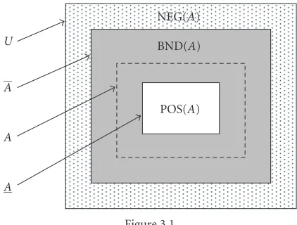
3.2. Decision-theoretic approach of rough sets (under equivalence relations). Let apr=(U,E) be an approximation space whereEis equivalence relation onU. With re-spect to a subsetA⊆U, one can divide the universeU into three disjoint regions, the positive region POS(A), the negative region NEG(A), and the boundary region BND(A) (seeFigure 3.1);
POS(A)=apr(A),
NEG(A)=U−A, BND(A)=apr(A)−apr(A).
(3.3)
NEG(A)
BND(A)
POS(A) U
A
A
[image:6.468.127.338.72.232.2]A
Figure 3.1
operators can be easily fitted into Bayesian decision-theoretic framework (Yao and Wong [1]). The set of states is given by Ω= {A,−A}indicating that an element is in Aand not inA, respectively. With respect to the three regions, the set of actions is given by Ꮽ= {a1,a2,a3}, wherea1,a2, anda3represent the three actions in classifying an object, deciding POS(A), deciding NEG(A), and deciding BND(A), respectively.
Letλ(ai/A) denote the loss incurred for taking actionaiwhen an object in fact belongs toA, andλ(ai/−A) denote the loss incurred for taking the same action when the object does not belong toA, the rough membership valuesμA(x)=P(A/[x]E) andμAC(x)=1− P(A/[x]E) are in fact the probabilities that an object in equivalence class [x]Ebelongs toA and−A, respectively. The expected lossR(ai/[x]E) associated with taking the individual actions can be expressed as
R a1 [x]E
=λ11P A [x]E
+λ12P −A [x]E
,
R a2 [x]E
=λ21P A [x]E
+λ22P −A [x]E
,
R a1 [x]E
=λ31P A [x]E
+λ32P −A [x]E
,
(3.4)
whereλi1=λ(ai/A),λi2=λ(ai/−A) andi=1, 2, 3.
The Bayesian decision procedure leads to the following minimum-risk decision rules: (P) ifR(a1/[x]E)≤R(a2/[x]E) andR(a1/[x]E)< R(a3/[x]E), decide POS(A);
(N) ifR(a2/[x]E)≤R(a1/[x]E) andR(a2/[x]E)< R(a3/[x]E), decide NEG(A); (B) ifR(a3/[x]E)≤R(a1/[x]E) andR(a3/[x]E)≤R(a2/[x]E), decide BND(A). Based onP(A/[x]E) +P(−A/[x]E)=1, the decision rules can be simplified by using only probabilitiesP(A/[x]E).
the loss of classifyingxinto the boundary region, and both of these losses are strictly less than the loss of classifyingxinto the negative region. For this type of loss functions, the minimum-risk decision rules (P)–(B) can be written as
(P) ifP(A/[x]E)≥γandP(A/[x]E)≥α, decide POS(A); (N) ifP(A/[x]E)< βandP(A/[x]E)≤γ, decide NEG(A);
(B) ifβ < P(A/[x]E)≤α, decide BND(A), where
α= λ12−λ32
λ31−λ32−λ11−λ12,
γ= λ12−λ22
λ21−λ22−λ11−λ12,
β= λ32−λ22
λ21−λ22−λ31−λ32.
(3.5)
From the assumptionsλ11≤λ31< λ21andλ22≤λ32< λ12, it follows thatα∈[0, 1],γ∈ (0, 1) andβ∈[0, 1). Note that the parametersλi jshould satisfy the conditionα≥β. This ensures that the results are consisted with rough set approximations. That is, the bound-ary region may be nonempty.
3.3. Generalized decision-theoretic approach of rough sets (under general relation). In fact, the original granulation of rough set theory based on partition is a special type of topological spaces. Lower and upper approximations in this model are exactly the closure and interior in topology. In general spaces, semiclosure and semiinterior (Crossley and Hildbrand [8]) are two types of approximation based on semiopen and semiclosed sets which are well defined (Levine [9]).
This fact with the concepts of semiclosure and semi-interior directed our intentions to introduce two new approximations. For any general binary relation, the general approxi-mations do not satisfy the properties (10, 11) inSection 2.1. Therefore, we can define two new approximations, namely, semilower and semiupper approximation.
Definition 3.1. Let apr=(U,E), whereEis any binary relation defined onU. Then we can define two new approximations, namely, semilower and semiupper approximations as follows:
semiL(A)=A∩Aβ
β,
semiU(A)=A∪Aβ
β.
(3.6)
The lower and upper approximations have the following properties.
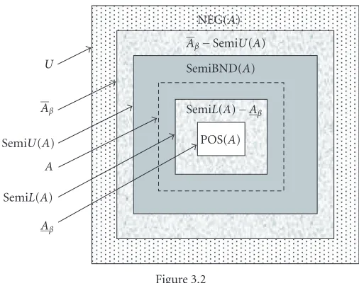
This definition enables us to divide the universeUinto five disjoint regions as follows (seeFigure 3.2):
POS(A), SemiL(A)−Aβ, SemiBND(A), Aβ−SemiU(A), NEG(A), (3.7) where,
SemiBND(A)=SemiU(A)−SemiL(A). (3.8)
In this case, the set of states remainsΩ= {A,−A}but the set of actions becomesᏭ= {a1,a2,a3,a4,a5}, wherea1,a2,a3,a4, anda5represent the five actions in classifying an object deciding POS(A), deciding SemiL(A)−Aβ, deciding SemiBND(A), decidingAβ− SemiU(A), and deciding NEG(A), respectively.
In an approximation space apr=(U,E), whereEis a binary relation, an elementxis viewed asβx(a subset of GKB containingx). Sinceβdoes not perform a partition onU in general, then we consider that∩βxbe a descriptionx. The rough membership values μA(x)=P(A/∩βx) andμAC(x)=1−P(A/∩βx) are in fact the probabilities that an object
in∩βx belongs toAand−A, respectively. The expected lossR(ai/∩βx) associated with taking the individual actions can be expressed as
R a1 βx
=λ11P A ∩βx
+λ12P −A ∩βx
,
R a2 βx
=λ21P A ∩βx
+λ22P −A ∩βx
,
R a3 βx
=λ31P A ∩βx
+λ32P −A ∩βx
,
R a4 βx
=λ41P A ∩βx
+λ42P −A ∩βx
,
R a5 βx
=λ51P A ∩βx
+λ52P −A ∩βx
.
(3.9)
The Bayesian decision procedure leads to the following minimum-risk decision rules. (1) If R(a1/∩βx)≤R(a2/∩βx), R(a1/∩βx)≤R(a3/∩βx), R(a1/∩βx)≤R(a4/
∩βx),R(a1/∩βx)≤R(a5/∩βx), decide POS(A).
(2) If R(a2/∩βx)≤R(a1/∩βx), R(a2/∩βx)≤R(a3/∩βx), R(a2/∩βx)≤R(a4/ ∩βx),R(a2/∩βx)≤R(a5/∩βx), decide SemiL(A)−Aβ.
(3) If R(a3/∩βx)≤R(a1/∩βx), R(a3/∩βx)≤R(a2/∩βx), R(a3/∩βx)≤R(a4/ ∩βx),R(a3/∩βx)≤R(a5/∩βx), decide Semi BND(A).
(4) If R(a4/∩βx)≤R(a1/∩βx), R(a4/∩βx)≤R(a2/∩βx), R(a4/∩βx)≤R(a3/ ∩βx),R(a4/∩βx)≤R(a5/∩βxβx), decideAβ−SemiU(A).
(5) If R(a5/∩βx)≤R(a1/∩βx), R(a5/∩βx)≤R(a2/∩βx), R(a5/∩βx)≤R(a3/ ∩βx),R(a5/∩βx)≤R(a4/∩βx), decide NEG(A).
NEG(A)
Aβ SemiU(A)
SemiBND(A)
SemiL(A) Aβ
POS(A) U
Aβ
SemiU(A)
A
SemiL(A)
[image:9.468.106.359.70.270.2]Aβ
Figure 3.2
Consider a special kind of loss function with
λ11≤λ21≤λ31≤λ41< λ51, λ52≤λ42≤λ32≤λ22< λ12. (3.10)
For this type of loss functions, the minimum-risk decision rules (1)–(5) can be written as follows.
(1) IfP(A/∩βx)≥b,P(A/∩βx)≥c,P(A/∩βx)≥d,P(A/∩βx)≥e, decide POS(A). (2) If P(A/∩βx)≤b, P(A/∩βx)≥ f, P(A/∩βx)≥g, P(A/∩βx)≥l, decide
SemiL(A)−Aβ.
(3) If P(A/∩βx)≤c, P(A/∩βx)≤ f, P(A/∩βx)≥m, P(A/∩βx)≥n, decide SemiBND(A).
(4) IfP(A/∩βx)≤d,P(A/∩βx)≤g,P(A/∩βx)≤m,P(A/∩βx)≥q, decideAβ− SemiU(A).
(5) IfP(A/∩βx)≤e,P(A/∩βx)≤l,P(A/∩βx)≤n,P(A/∩βx)≤q, decide NEG(A) where
b= λ12−λ22
λ21−λ22−λ11−λ12,
c= λ12−λ32
λ31−λ32−λ11−λ12,
d= λ12−λ42
λ41−λ42−λ11−λ12,
e= λ12−λ52
f = λ22−λ32
λ31−λ32−λ21−λ22,
g= λ22−λ42
λ41−λ42−λ21−λ22,
l= λ22−λ52
λ51−λ52−λ21−λ22,
m= λ32−λ42
λ41−λ42−λ31−λ32,
n= λ32−λ52
λ51−λ52−λ31−λ32,
q= λ42−λ52
λ51−λ52−λ41−λ42.
(3.11)
A loss function should be chosen in such a way to satisfy the conditions:
b≥f, b≥g, b≥l c≥m, c≥n, f ≥m, f ≥n
q≤d, q≤g, q≤m.
(3.12)
These conditions imply that (SemiL(A)−Aβ)∪SemiBND(A)∪(Aβ−SemiU(A)) is not empty, that is, the boundary region is not empty.
Example 3.2. InExample 2.1, we choose any subsetAfromU, say
A=x1,x3,x4,x6. (3.13)
Now, we can decide the region for each object by using the generalized decision-theoretic approach that proposed inSection 3.3. This approach can be applied on a mul-tivalued information system and gives us the ability to divide the universeUinto five re-gions which help in increasing the decision efficiency. The result given by general rough sets model can be viewed as a special case of our generalized approach.
In our example, the set of states is given byΩ= {A,−A}indicating that an element is inAand not inA, respectively. With respect to five regions, the set of actions is given by Ꮽ= {a1,a2,a3,a4,a5}.
To apply our proposed technique, consider the following loss function:
λ11=λ52=0, λ21=λ42=0.25, λ31=λ32=0.5,
λ41=λ22=1, λ51=λ12=2. (3.14)
Table 3.1
P(A/∩βx) Decision
x1 1 POS(A)
x2 0.75 SemiL(A)−Aβ
x3 1 POS(A)
x4 0.25 Aβ−SemiU(A)
x5 0 NEG(A)
x6 1 POS(A)
x7 0 NEG(A)
x8 0 NEG(A)
x9 0 NEG(A)
x10 0.5 Semi BND(A)
an object into boundary region, and 1 unit cost for classifying an object belong toAinto Aβ−SemiU(A) and for an object does not belong toAinto SemiL(A)−Aβ(note that a loss function supplied by user or expert). According to these losses, we have
b=0.8, g=0.5, c=0.75, l=0.36, d=0.64, m=0.33, e=0.5, n=0.25,
f =0.67, q=0.2.
(3.15)
By using the decision rules (1)–(5), we get the results shown inTable 3.1. Thus, we have
POS(A)=x1,x3,x6,
SemiL(A)−Aβ=x2,
SemiBND(A)=x10,
Aβ−SemiU(A)=
x4,
NEG(A)=x5,x7,x8,x9.
(3.16)
Now we apply the decision theoretic technique proposed by Yao and Wong [1] to clas-sify the decision region into three areas. The set of actions is given byᏭ= {a1,a2,a3}, wherea1,a2, anda3represent the three actions in classifying an object, deciding POS(A), deciding NEG(A), and deciding BND(A), respectively. To make this, consider that there is 0.25 unit cost for a correct classification, 3 units of cost for an incorrect classification, and 0.5 unit cost for classifying an object into boundary region, that is,
Table 3.2
P(A/∩βx) Decision
x1 1 POS(A)
x2 0.75 BND(A)
x3 1 POS(A)
x4 0.25 BND(A)
x5 0 NEG(A)
x6 1 POS(A)
x7 0 NEG(A)
x8 0 NEG(A)
x9 0 NEG(A)
x10 0.5 BND(A)
These losses give us that
α=0.9, γ=0.5, β=0.1. (3.18)
By using the decision rule (P)–(C) and replacingP(A/[x]E) byP(A/βx), we get the results shown inTable 3.2.
This means that
POS(A)=x1,x3,x6,
BND(A)=x2,x4,x10,
NEG(A)=x5,x7,x8,x9.
(3.19)
From the comparison between the two approaches, we note that the our approach (classification of decision region into five areas) gives us the ability to divid BND(A)= {x2,x4,x10} into SemiL(A)−Aβ = {x2}, which is closer to the positive region, Aβ− SemiU(A)= {x4}, which is closer to the negative region, and Semi BND(A)= {x10}.
4. Conclusion
The decision theoretic rough set theory is a probabilistic generalization of standard rough set theory and extends the application domain of rough sets. The decision model can be interpreted in terms of more familiar and interpretable concept known as loss or cost. One can easily interpret or mesure loss or cost according to real application.
References
[1] Y. Y. Yao and S. K. M. Wong, “A decision theoretic framework for approximating concepts,”
International Journal of Man-Machine Studies, vol. 37, no. 6, pp. 793–809, 1992.
[2] Z. Pawlak, “Rough sets,” International Journal of Computer and Information Sciences, vol. 11, no. 5, pp. 341–356, 1982.
[3] E. A. Rady, A. M. Kozae, and M. M. E. Abd El-Monsef, “Generalized rough sets,” Chaos, Solitons
and Fractals, vol. 21, no. 1, pp. 49–53, 2004.
[4] Z. Pawlak and A. Skowron, “Rough membership functions,” in Advances in the Dempster-Shafer
Theory of Evidence, R. R. Yager, M. Fedrizzi, and J. Kacprzyk, Eds., pp. 251–271, John Wiley &
Sons, New York, NY, USA, 1994.
[5] E. F. Lashin, A. M. Kozae, A. A. Abo Khadra, and T. Medhat, “Rough set theory for topological spaces,” International Journal of Approximate Reasoning, vol. 40, no. 1-2, pp. 35–43, 2005. [6] M. M. E. Abd El-Monsef, Statistics and Roughian, Ph.D. thesis, Faculty of Science, Tanta
Univer-sity, Tanta, Egypt, 2004.
[7] R. O. Duda and P. E. Hart, Pattern Classification and Scene Analysis, John Wiley & Sons, New York, NY, USA, 1973.
[8] S. G. Crossley and S. K. Hildbrand, “Semi-closure,” Texas Journal of Science, vol. 22, no. 2-3, pp. 99–119, 1971.
[9] N. Levine, “Semi-open sets and semi-continuity in topological spaces,” The American
Mathe-matical Monthly, vol. 70, no. 1, pp. 36–41, 1963.
M. M. E. Abd El-Monsef: Department of Mathematics, Faculty of Science, Tanta University, Tanta 31527, Egypt
Email address:[email protected]
N. M. Kilany: Commercial Technical Institute for Computer Sciences, Suez, Egypt