Approximate solution for Euler equations of stratified water via numerical solution of coupled KdV system

PII. S0161171203212242 http://ijmms.hindawi.com © Hindawi Publishing Corp.

APPROXIMATE SOLUTION FOR EULER EQUATIONS

OF STRATIFIED WATER VIA NUMERICAL

SOLUTION OF COUPLED KdV SYSTEM

A. A. HALIM, S. P. KSHEVETSKII, and S. B. LEBLE

Received 23 December 2002

We consider Euler equations with stratified background state that is valid for in-ternal water waves. The solution of the initial-boundary problem for Boussinesq approximation in the waveguide mode is presented in terms of the stream func-tion. The orthogonal eigenfunctions describe a vertical shape of the internal wave modes and satisfy a Sturm-Liouville problem. The horizontal profile is defined by a coupled KdV system which is numerically solved via a finite-difference scheme for which we prove the convergence and stability. Together with the solution of the Sturm-Liouville problem, the stream functions give the internal waves profile. 2000 Mathematics Subject Classification: 76B15, 76B70, 76B55, 37L65, 65M06, 65M12.

1. Introduction. The basic system of Euler equations for internal water waves in two dimensions(xz), with a stable stratified ambient state and the buoyancy frequencyN(z), is

ux+wz=0,

ρout= −ρo _→

v ,→∇ u−px,

ρowt= −ρo _→

v ,→∇w−pz−ρg,

Tt+wT¯z= − _→

v ,→∇ T,

(1.1)

whereu,vare velocity components,ρois the density,pis the pressure,ρgis the body force due to stratification, ¯Tzis the vertical background temperature gradient, andTis the temperature variable [3]. Combining the equations in (1.1) and using the state relation for liquidρ= −ρoαT,α= −ρz/(ρT¯z)is the coefficient of thermal expansion, and ¯Tz=N2/(αg), we obtain

∆wtt+N2wxx−N2 _→

v ,→∇ t

0w dt

xx

+→v , →∇ wzdx

txz+ _→

v ,→∇ w_txx=0.

Rescaling the dimensionless variables (primed) usingxi=λixi,t=2π t/Nβ,¯ u=λzNu¯ /2π, w=βλzNw¯ /2π, αT=T, N=NN¯ /2π, ¯N is the average buoyancy frequency andβis a scale parameter. Substitute in (1.2) and omit primes for simplicity to obtain

λz _Nβ¯

2π 3_w

xx λ2

x + wzz

λ2 z tt+

_N¯

2π 3

(βN)2 _w

xx λx

−

_N¯

2π

3_(βN)2

λx u

t

0

wxdt+w t

0 wzdt

xx

+

_Nβ¯

2π 3

λλ2xz

uwx+wwz

xxt

+_λ1 z

uwz+w t

0 wzdx

z

xzt   =0.

(1.3)

Introduce the stream functionψ, w= −σ ψx andu=σ ψz(σ is a scale pa-rameter). Integrate, with respect tox,

ψzztt+N2ψxx= −β2ψxxtt−σψzψxz−ψxψzzzt

+σ N2

ψz t

0ψxxdt−ψx t

0ψxzdt

x.

(1.4)

Substitute in (1.4) by the stream function of the form

ψ(z, x, t)= m

Zm_(z)θm_{(x, t), (1.5)}

multiply byZn_{, integrate with respect toz, and use the separation of variables} that give

Zn zz= −

N2 c2

n

Zn_{. (1.6)}

So (1.4) becomes

θttn−cn2θxxn

=cn2β2 N2 θ

n

xxtt+σ cn2

m,k

an m,k

θm_θk

x

t+

bn

m,kθmθkt+enm,kθxm t

0 θk

xdt

x

,

where

an_m,k=N2 h

−h

−1 c_k2+

1 c2m

zzmzkzndz, bnm,k= −N2

c_k2 h

−hz m

zzkzndz,

en_m,k=N2 h

−hz m_zk

zzndz.

(1.8)

System (1.7) describes the two oppositely directed propagated modes. The equations of the separated propagated modes are obtained by substituting θn

t =un,cnθxn=vn, so (1.7) becomes

unt −cnvxn= c3

nβ2 N2 v

n

xxx+σ c2n

m,k   anm,k

t

0u

m_dt·vk ck

t

+

bn_m,k

t

0u

m_dt·uk_+en m,k vm cm t 0 vk ck dt x   ,

vtn−cnunx=0.

(1.9)

Using projection operators,

P+=1₂

   

1 1+c_2N2β₂2∂2 x

1−c_2N2β22∂ 2 x 1    ,

P₋=1

2    

1 −1−c2β2

2N2∂ 2 x

−1+c_2N2β₂2∂2

x 1    . (1.10) So P+ un vn = ϕn+

kϕn+

, P−

un vn = ϕn−

−kϕn−

(1.11)

or

un_=ϕn+_+ϕn−_{, v}n_=ϕn+_−ϕn−₋c2β2

2N2∂ 2 x

ϕn+_−ϕn−_{. (1.12)}

Operating P₊, P₋ on (1.9) and using (1.12), we obtain the equations for the separated modesϕn+_,ϕn−_as

ϕtn+−cnϕnx+− c3_β2

2N2ϕ n+

xxx− σ c2

n 2

m,k an_m,k

t

0

ϕ++ϕ−mdt·

ϕ+−ϕ−k ck t + bn m,k t 0

ϕ++ϕ−mdt·ϕ++ϕ−k

+en m,k

ϕ+−ϕ−m cm

t

0

ϕ+−ϕ−k ck

dt

ϕtn−+cnϕnx−+ c3_β2

2N2ϕ n−

xxx− σ c2

n 2

m,k an_m,k

t

0

ϕ++ϕ−mdt·

ϕ+−ϕ−k ck

t

+

bn

m,k t

0

ϕ++ϕ−mdt·ϕ++ϕ−k

+en m,k

ϕ+−ϕ−m cm

t

0

ϕ+−ϕ−k ck

dt

x

=0. (1.13)

Letϕn+_=ηn+

t ,ϕn−=ηnt−, so (1.13) becomes

ηnt+−cnηnx+= c3_β2

2N2η n+

xxx+ σ c2

n 2

m,k

an_m,kη++η−mη+−η−k_x

+bnm,k

η++η−m·η++η−kx

+ e n m,k ckcm

η+−η−m_xη+−η−k,

ηnt−+cnηnx−= − c3_β2

2N2η n−

xxx+ σ c2

n 2

m,k anm,k

η++η−mη+−η−kx

+bn m,k

η++η−m·η++η−k_x

+ e n m,k ckcm

η+−η−mx

η+−η−k.

(1.14)

In what follows we will consider both directed modes. In this work we eval-uate only for short time to describe the phenomena, so we consider only one direction of the propagating modes. Hence the system that describes one di-rection of (1.7) has the form (return toθvariable for convenient)

θnt+cnθxn+σ

m,k

gm,kn θmθxk+β2dnθnxxx=0, (1.15)

gnm,k= σ N2_c2

n 2

h

−h

−1 cm2 +

2 c2k

ZkZzm−

1 cmck

ZmZzk

Zndz, dn= c3

n 2N2.

(1.16)

2. Physical model. In this model, we simulate the initial stage of McEwan experiment [4,5] for a rectangular tank of dimension 50 cm inxby 25 cm inz directions filled by a linearly stratified water of constant buoyancy frequency 1.23s−1_{. The internal water waves are described by system (1.1). The solution} of this system is constructed as the representation for the stream function (1.5), whereZn_{(z)are solutions of the correspondent Sturm-Liouville problem} (1.6),Zzz+(N2/cn2)Z=0,Z(0)=Z(h)=0, and describe a vertical shape of the wave modes. The linear propagation velocitiescnplay the role of eigenvalues. The coefficient functions θn_{(x, t) are solutions of the coupled KdV system} (1.15) with coefficients from (1.16). We select a localized initial condition along x-axis described by a smooth enough function that models the paddle motion as in the experiments of McEwan [5]. The function is also chosen antisymmetric alongx-axis in relation to the paddle axis centered in the middle of the tank. The time intervals of simulations are taken such that the initial disturbance decays essentially but does not reach the boundaries.

3. Computation. When the coefficients in the Sturm-Liouville equation (1.6) are constant, it has very simple general solution

Zn_=B nsin

_{nπ z}

h , n=1,2,3, . . . , L, (3.1)

which tends to zero at boundaries. The eigenvalues

cn= Nh

nπ, n=1,2,3, . . . , L, (3.2)

have the sense of linear internal gravity waves velocities. Normalization is de-termined by₀h(Zn₎2_N2_{dz=1 and givesB}

n=(2/N2h)1/2. Hence

Zn(z)=

₂

N2_h 1/2

sin _{nπ z}

h . (3.3)

To solve the coupled KdV system (1.15) an initial condition is required. We can select the initial perturbation for the stream function (1.5) which has the general form

ψ(z, x,0)= L

n=1

Zn_(z)θn_{(x,0)=ϕ(x, z)=ϕ}

1(x)ϕ2(z). (3.4)

ϕ1(x)= a cosh(x/l),

ϕ2(z)=

₂

N2_h 1/2

sechbz−z0

tanhbz−z0

,

(3.5)

as the initial condition we model the impact of a wave-productor.

The choice of the form and the constantsa, b,lqualitatively reflects the paddle movement (we restrict the movement by some isolated pulse), and the numerical value for the amplitude is estimated also from the description of the experiment of McEwan [5]. Then the scalar product gives

Zj, ψ= L

n=1

Zj, Znθn(x,0)=Zj, ϕ2(z)

ϕ1(x), (3.6)

Zj_{, ϕ}

2(z)= h

0

N2_Zj_ϕ

2(z)dz, (3.7)

and using the orthogonality,

Zj, Zn=

h

0N

2_Zj_Zn_{dz=1, (j=n),0, (j≠n). (3.8)}

Hence, (3.6) givesθn_{(x,0), the initial condition of system (1.15) which is solved} by the numerical method introduced below.

4. Numerical method. For the coupled KdV system (1.15) we introduce a numerical (finite-difference) method of solution, a two-step three-time-level scheme similar to the Lax-Wendroff one [1,7]. The usual Lax-Wendroff scheme is modified such that the order of the first derivative becomes of orderO(x4_). The approximation of the nonlinear terms is changed such that the integral of θ2_{is a conserved one. The scheme has the form}

θnj+1/2

i −

θnj

i !

τ/2 +

cn θnji+1−

θnj i−1

!

2h

+

k,m gn

mk

θmj i

θkj i+1−

θkj

i−1 !

2h

+

dn−

cnh2 6

θnj i+2−2

θnj

i+1+2

θnj i−1−

θnj

i−2 !

2h3

=0,

(4.1)

for the intermediate layer as

θnj+1

i −

θnj

i !

τ +

cn θnji++11/2−

θnj+1/2 i−1

!

2h

+

k,m gnmk

θmji+1/2

θkj+1/2 i+1 −

θkj+1/2 i−1

!

2h

+en θ nj+1/2

i+2 −2

θnj+1/2 i+1 +2

θnj+1/2 i−1 −

θnj+1/2 i−2

!

2h3 =0.

(4.2)

To support the results, we prove stability and convergence of the scheme in AppendicesAandB[2]. Beside these proofs, we would like to mention that the order of errors of the difference formulas is improved at the same time they preserve conservation laws of the KdV-type equations [6].

5. Results. Figure 5.1is a contour plot presenting the initial perturbation ψ(z, x,0)for the upper half of the tank due to antisymmetry.

Figure 5.2is one-dimensional(x)plots for the second tenth modes.

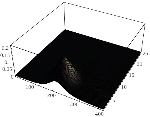
Figure 5.3is a three-dimensional plot for the wave profile (1.5) att=0.02 second for the same half of the tank.

100

200

300

400 5

10 15

20 25

0 0.05

0.1 0.15

0.2

−0.07

−0.05

−0.03

−0.01 0.01

0.25 0.15 0.05

−0.05

−0.15

−0.25

x-axis

Second mode, series 1(t=0), series 2(t=0.02 s) Series 1

Series 2

−0.01 0.01 0.03 0.05 0.07

0.25 0.15 0.05

−0.05

−0.15

−0.25

x-axis

Fourth mode, series 1(t=0), series 2(t=0.02 s) Series 1

Series 2

−0.07

−0.05

−0.03

−0.01 0.01

0.25 0.15 0.05

−0.05

−0.15

−0.25

x-axis

Sixth mode, series 1(t=0), series 2(t=0.02 s) Series 1

Series 2

−0.01 0.01 0.03 0.05 0.07

0.25 0.15 0.05

−0.05

−0.15

−0.25

x-axis Eighth mode, series 1(t=0),

series 2(t=0.02 s) Series 1

Series 2

−0.07

−0.05

−0.03

−0.01 0.01

0.25 0.15 0.05

−0.05

−0.15

−0.25

x-axis

Tenth mode, series 1(t=0), series 2(t=0.02 s) Series 1

Series 2

100

200

300

400 5

10 15

20 25

0 0.2 0.4

Figure _5.3. _{Three-dimensional (x, y, z) plot of the wave profile} ψ(z, x, t)att=0.02 second for the upper half of the tank. The hor-izontal numbers(25,400)indicate the number of mesh points used in plotting inxandzdirections while the dimensions are 12.5 cm inzand 50 cm inx, respectively.

All the plots for the modes and for the sum (stream function) show the be-havior that is typical for the multisolitonic perturbation. It looks like a decay of the initial condition to solitons in the single KdV equation theory. The process of the wave propagation is accompanied by interaction that implies the energy transfer between modes. This phenomenon may be considered as a possible reason for the vertical fine-structure generation [3]. The combination of the fine structures may explain McEwan experiments [4,5].

6. Summary. In the commonly accepted approximations (incompressibil-ity, Boussinesq approximation, and so forth), the solution of the system of Euler equations with stratified background state is constructed as the repre-sentation for the stream function. The horizontal profile is defined by a cou-pled KdV system which is numerically solved via a finite-difference scheme for which stability and convergence are proved. Together with the solution of the Sturm-Liouville problem that describes the vertical profile, the stream function gives the complete internal waves profile.

Appendices

perturbation of the initial data. Consider the differential

Ti,rn,j+1=

"_∂θn,j+1 i ∂θrn,j

# ,

dθn,jr = θ_in,j₋₂ θ_in,j₋₁ θ_in,j θ_in,j₊₁ θ_in,j₊₂ !t

(A.1)

and define the norm

$$dθj$$₌ 



r

n

dθrn,j2h  

1/2

. (A.2)

We can write

dθn,j_i +1=T_i,rn,j+1dθn,jr =Ti,rn,j+1T n,j i,r dθ

n,j−1

r =Πr

T_i,rnrdθn,o

r , (A.3)

wheredθ_in,j+1is the perturbation of the discrete solution anddθn,or is a small perturbation of the initial data. Stability required the boundness ofΠr(Tn

i,r)r, that is,Tr_{is bounded. We calculateTfrom the difference scheme as follows:}

T_i,rn,j+1=δi,r− cnτ

2h

δi+1,r−δi−1,r

−τ m,k

gnm,k

2h %

θm,ji

δi+1,r−δi−1,r

+δi,r

θik,j+1−θ k,j i−1

&

−τen 2h3

δi+2,r−2δi+1,r+2δi−1,r−2δi−2,r

.

(A.4)

Rewriting the matrixT (A.4) in terms of identity(E), symmetric(S), and anti-symmetric(A), matrices yieldsT=E+S+A,

Sn,j+1

i,r= − τ 4h

m,k gn

m,k %

θ_im,j−θm,j_i+1δi+1,r−

θm,j_i −θ_im,j₋₁δi−1,r

+2δi,rθk,ji+1−θ k,j i−1

& ,

An,j+1

i,r= − cnτ

2h

δi+1,r−δi−1,r

−_4hτ m,k

g_m,kn %θ_im,j+θm,j_i+1δi+1,r−

θ_im,j+θm,j_i−1δi−1,r &

−enτ 2h3

δi+2,r−2δi+1,r+2δi−1,r−δi−2,r,

$$_Sj+1$$_≤τmax n,m,k

''_gn m,k''max

i,m,k ''_θm,j

θm,j_x,i =

θim,j+1−θ

m,j i

h , θ` k,j x,i=

θik,j+1−θ

k,j i−1

2h , $$Aj+1$$_≤τmaxn,m,k''g

n m,k'' h maxm,i

''θ_im,j''+τmaxn''cn''

h +

3τmaxn''en'' h3 , $$Tj+1$$2=$$$Tj+1∗Tj+1$$$=$$E−Aj+1+Sj+1E+Aj+1+Sj+1$$

≤1+2$$Sj+1$$₊$$_Aj+1$$₊$$_Sj+1$$2

≤1+2τmax n,m,k

''gn m,k''max

m,i ''θ_x,im,j''

+τ2

max n,m,k

''gn m,k''max

m,i

''θm,j_x,i''+maxn,m,k''g n m,k'' h maxm,i

''θm,j_i ''

+maxn''cn''

h +

3 maxn''en'' h3

2

≤eaτ,

a=1+2τmax n,m,k

''gn_m,k''max m,i

''θ_x,im,j''

+τ2

max n,m,k

''_gn

m,k''max_m,i ''θ m,j x,i''+

maxn,m,k''gnm,k'' h maxm,i

''_θm,j i ''

+maxn''cn''

h +

3 maxn''en'' h3

2 ,

(A.5)

which is a necessary condition of stability. The scheme is stable ifa≤constant in spite ofτ,h→0. This is a conditional stability of the scheme. It means that it is required for stability thatτ→0 more faster thanh→0 or

τ≤(constant)·h6_{. (A.6)}

B. Convergence proof of the scheme. We would prove that the solution of the difference equations (4.1) and (4.2) converges to the solution of (1.15) if the exact solution is a continuously differentiable one. We place here for brevity a proof that uses only one-step time difference equation and the whole proof may be developed by similar ideas. Therefore, we now consider the difference equation

θnj+1

i −

θnj

i τ +cn

θnj

i+1−

θnj i−1 2h +

m,k

gn_m,kθmji

θkj i+1−

θkj

i−1 2h

+en

θnj i+2−2

θnj

i+1+2

θnj i−1−

θnj

i−2 2h3 =0.

We know that the KdV-type equation has the conservation law_−∞∞ u2_{(x, t)dx=} constant. It may also be shown that if a smooth enough solutionun_{(x, t)of} the set of equations (1.15) exists, then it satisfies the inequality(L_n=1−∞∞ (un_(x, t))2_{dx < B, for a finitet, whereBis a constant dependent on initial conditions} only,L-number of modes taken into account by system (1.15). Therefore, it is natural to useL2-norm in the proof, and

$$_Θj$$₌   i n %

θn2h&j i  

1/2

. (B.2)

Here,his a grid step,iis a discrete space variable, andjis the discrete time. The symbolΘ denotes a columnΘj _≡(θ1₎j _(θ2₎j _(θ3₎j _···t _{and the} components of this column are columns also:

θnj≡ ··· θnj i−1

θnj

i

θnj i+1 ···

!t

, (B.3)

where(θn₎j

i is a solution of the finite-difference equation (B.1). Let the vector(un₎j

i=un(xi, tj)be an exact solution of (B.1) in the points of grid. Then the error(vn₎j

i is given by

vnji=

θnji−

unji. (B.4)

The difference solution(θn₎j

iconverges to the exact solution(un) j

iifVj →0 asτ, h→0, whereVj_≡Θj_−Uj_{. Substitute (B.4) into (B.1) and obtain}

vnj+1

i −

vnj

i τ +cn

vnj

i+1−

vnj i−1 2h

+ m,k

gm,kn

umji

vkj i+1−

vkj

i−1 2h +g

n m,k

vmji

ukj

i+1−

ukj i−1 2h

+gn m,k

vmj

i

vkj i+1−

vkj

i−1 2h

+en

vnj i+2−2

vnj

i+1+2

vnj i−1−

vnj

i−2 2h3

= − un

j+1

i −

unj

i τ +cn

unj

i+1−

unj i−1 2h

+ m,k

gm,kn

umji

ukj i+1−

ukj

i−1 2h

+en

unj i+2−2

unj

i+1+2

unj i−1−

unj

i−2 2h3

.

Pick out (inv) a linear part of expression (B.5) and introduce for convenience an operatorTj_{by the expression}

vnji−τ  cn

vnj

i+1−

vnj i−1 2h

m,k

g_m,kn umji

vkj i+1−

vkj

i−1 2h

+gm,kn

vmji

ukj i+1−

ukj

i−1 2h

+en

vnj i+2−2

vnj

i+1+2

vnj i−1−

vnj

i−2 2h3

 

= r

Tj+1ir

vnji, n=1,2,3, . . . , L.

(B.6)

Using the above expression forT and utilizing that(un₎j

iis an exact solution of differential equations, due to the approximation, we use the fact that the right-hand-side term of (B.5) is a small one of orderO(τ+h2_{). Therefore, we} can rewrite (B.5) as follows:

vnj+1

i −

r

Tj+1 ir

vnj

i

+τ m,k

gm,kn

vmji

vkj i+1−

vkj

i−1 2h =O

τ+h2

(B.7)

or

vnji+1=

r

(Tj+1)ir

vnji+τ

fn,m,kji, (B.8)

where

fnmkj

i= −τ

m,k gn

m,k

vmj i

vkj i+1−

vkj

i−1 2h +O

τ+h2_{, (B.9)}

and the following estimation for the norm is valid:

$$Vj+1$$≤$$Tj+1$$$$Vj$$+τ$$fj$$. (B.10)

If we will consequently substitute (B.10) into itself, we will get $$vj+1$$_≤$$_Tj+1$$$$_vj$$_+τ$$_fj$$

≤$$Tj+1$$$$_Tj$$$$_vj−1$$_+τ$$_Tj+1$$$$_fj−1$$₊$$_fj$$ ≤$$Tj+1$$$$Tj$$$$Tj−1$$$$vj−2$$

+τ$$Tj+1$$$$Tj$$$$fj−2$$+$$Tj+1$$$$fj−1$$+$$fj$$.

Using the estimate of norm ofT in inequality (A.5), (B.11) becomes $$_vj+1$$_≤eaτj$$_v0$$_+τeaτ(j−1)$$_f0$$_+eaτ(j−2)$$_f1$$_+···$$_fj$$

≤eaτj$$v0$$+Mmax k≤j

$$_fk$$_{, M=τ}eatmax−1 eaτ₋₁ ;

(B.12)

Mis the sum of a geometric series andtmaxis the time of simulation, 0≤t≤ tmax. The norm of(fn,m,k)

j

i is given by simple estimations

$$fj$$=

 

i %

fmkji &2

h  

1/2

=max n,m,k

''gn_m,k''  



i 



m,k

vmj i

vkj i+1−

vkj

i−1 2h

  2

h   

1/2

≤max n,m,k

''gn m,k''





i

m %

vmj i

&2 h

i

k %

vkj i

&2 h

 

1/2 1 h3/2

≤maxn,m,k''g n m,k'' h3/2 $$V

j$$2

+Oτ+h2.

(B.13)

Using this estimate in inequality (B.12) yields

$$_Vj+1$$_≤eaτj$$_V0$$_+M

maxn,m,k''gnm,k'' h3/2 $$V

j+1$$2

+Oτ+h2

. (B.14)

Taking into considerationV0 _{=0, the above inequality gives the solution}

$$Vj+1$$_≤1−

-1−4Mmaxn,m,k''gnm,k''/h3/2

MOτ+h2

2Mmaxn,m,k''gm,kn ''/h3/2 MOτ+h2_,

(B.15)

that is,Vj+1 _{→0 asτ, h→0. Hence the convergence is proved.}

Acknowledgment. This work was partially supported by the KBN Grant no 5 PO3B 040 20.

References

[1] S. P. Kshevetskii,Analytical and numerical investigation of nonlinear internal grav-ity waves, Nonlinear Processes in Geophysics8(2001), 37–53.

[2] P. Lancaster,Theory of Matrices, Academic Press, New York, 1969.

[3] S. B. Leble,Nonlinear Waves in Waveguides: with Stratification, Springer-Verlag, Berlin, 1991.

[4] A. D. McEwan,Internal mixing in stratified fluids, J. Fluid Mech.128(1983), 59–80. [5] ,The kinematics of stratified mixing through internal wavebreaking, J. Fluid

[6] Z. Shaohong,A difference scheme for the coupled KdV equation, Commun. Nonlin-ear Sci. Numer. Simul.4(1999), no. 1, 60–63.

[7] J. C. Tannehill, D. A. Anderson, and R. H. Pletcher,Computational Fluid Mechanics and Heat Transfer, Taylor & Francis, Washington, 1997.

A. A. Halim: Theoretical and Mathematical Physics Department, Gdansk University of Technology, 80-952 Gdansk, Poland

E-mail address:[email protected]

S. P. Kshevetskii: Theoretical Physics Department, Kaliningrad State University, Kalin-ingrad 236041, Russia

E-mail address:[email protected]

S. B. Leble: Theoretical and Mathematical Physics Department, Gdansk University of Technology, 80-952 Gdansk, Poland