M icrosim ulation and analysis o f incom e
distribution: an application to Italy
by
Carlo V. Fiorio
A thesis submitted for the degree of Doctor of Philosophy of the
University of London
Department of Economics
London School of Economics and Political Science
UMI Number: U61BB52
All rights reserved
INFORMATION TO ALL USERS
The quality of this reproduction is dependent upon the quality of the copy submitted. In the unlikely event that the author did not send a complete manuscript and there are missing pages, these will be noted. Also, if material had to be removed,
a note will indicate the deletion.
Dissertation Publishing
UMI U613352
Published by ProQuest LLC 2014. Copyright in the Dissertation held by the Author. Microform Edition © ProQuest LLC.
All rights reserved. This work is protected against unauthorized copying under Title 17, United States Code.
ProQuest LLC
789 East Eisenhower Parkway P.O. Box 1346
| L ib ^ r y
British >J»* *uut»
1 and Econom* *whk*
7 H £ £ £ S
I'
E S I 2.
-ABSTRACT
The first chapters of the thesis put special emphasis on tax-benefit microsimulation models. The state of the art in the economic literature of tax-benefit microsimula tion models is reviewed and discussed. Particular attention is paid to issues such as the reliability of estimation and the grossing-up of the sample. In order to anar lyze tax-benefit microsimulation, a new model is developed focusing on the case of Italy: it shares many features with other country-specific tax-benefit microsimulation models. The model, appropriately calibrated to population totals, is also used for an estimation of tax evasion via comparison with a number of different data sources. Non-parametric density estimation is used to improve the understanding of policy simulations and to analyze the effect of fiscal reform: an application to the 1998 Italian personal income taxation reform is provided. The first part concludes with an analysis of the reliability of microsimulation models, which has been addressed by few authors before. The analysis is undertaken using the bootstrap, which tends to show a better performance in finite sample than asymptotic approximations. The main result is that static microsimulation does not by itself make confidence intervals larger: on the contrary they can also make it smaller. To improve the reliability of microsimulation models the best way to proceed is to reduce the sampling ..error of the available data sets.
ACKNOWLEDGMENTS
It has been a privilege for me to spend these past years at the London School of Economics. I have greatly benefited from the courses I took, the seminars I attended, the researchers I interacted with. There are many people I would like to thank for their advice, feedback and support, without whom this thesis may not have come about.
I am truly indebted to Frank Cowell for his careful supervision, support, and great patience over the past five years. It was through him that I received access to the office facilities in STICERD, a resource that proved invaluable to my research.
Vassilis Hajivassiliou also provided thoughtful supervision, his insights and help with Chapter 7 are particularly appreciated.
I acknowledge financial support from ESRC, STICERD, ONAOSI, Universita di Milano, Universita di Padova, Universita di Pavia, for which I am thankful.
I would also like to thank the Bank of Italy for providing me with the Survey of Household of Income and Wealth data set.
Further thanks go to Roberto Artoni for his continued support. Sanghamitra Bandyopadhyay, Andrea Brandolini, Conchita D’Ambrosio, Joanna Gomulka, Fab- rizio Iacone, Marco Manacorda, Daniela Mantovani, Ceema Namazie for their gener ous gifts of time and useful comments.
Emmanuel Flachaire patiently introduced me to the bootstrap which plays a rel evant role in these thesis. How many times since have I had to let you win at squash? Frederic Robert-Nicoud helped me put the world to rights over numerous frozen pizzas as we shared the LSE experience. Marco Piersimoni for his polite humor and great cooking. Tim Walker for his immediate friendship, the scars from frisbee matches remain. The LSE would have not been such a pleasant working environment - and London not such a pleasant place to live in - without the company of Heski Bar-Isaac, Ralph Bayer, Sabine Bernabe and Anders, Virginie Blanchard, Thomas Buettner, Chiara Candelise, David Chilosi, Paolo Cossu, Guillermo Cruces, Juan De Laiglesia, M arta Foresti, Sinead Lester, Pete Longyear, Jez Longyear, Rocco Macchi- avello, Maryla and Wojtek Maliszewski, Maria Luisa Mancusi, Felix Muennich, Silvia Pezzini, Michele Pellizzari, Amedeo and Annarita Poli, Riccardo Puglisi, Annamaria Reforgiato-Recupero, Toril Skjetne, Cecilia Testa, among many others.
Table o f C ontents
1 M icrosimulation: a tool for econom ic analysis 1
1.1 Microsimulation in eco n o m ic s... 2
1.2 Static microsimulation m o d e ls... 7
1.2.1 Static microsimulation models with behavioral responses . . . 9
1.3 Dynamic microsimulation m o d e ls ... 10
1.3.1 Dynamic cross-section microsimulation m o d els... 11
1.3.2 Dynamic longitudinal microsimulation m o d e ls ... 12
1.3.3 Limitations of dynamic microsimulation m o d e ls ... 13
1.4 Issues in microsimulation m odelling... 14
1.4.1 G rossing-up... 14
1.4.2 V alid atio n ... 17
1.4.3 R eliab ility ... 18
1.5 Conclusion... 20
2 A static tax-benefit m icrosim ulation m odel for Italy 22 2.1 The data set for Italian M SM s... 23
2.1.1 Some limitations of the d a t a b a s e ... 25
2.2 Structure of the m o d e l... 26
2.3 Building the tax b a s e ... 29
2.4 G ro ssin g -u p ... 31
2.5 Estimation of tax evasion and v a lid a tio n ... 39
3 M icrosim ulation and non-param etric estim ation 46
3.1 The data set, the microsimulation model and the IRPEF reform . . . 48
3.2 The density estimation te c h n iq u e ... 50
3.3 The non-parametric density estimation and the MSM combined using co u n te rfac tu a ls... 53
3.3.1 Decomposing the s a m p le ... 56
3.3.2 Losers and g a i n e r s : . 59 3.4 A revenue-neutral reform sim ulation... 62
3.5 Decomposing the fiscal re fo rm ... 66
3.6 C on clu sio n s... 71
3.7 Appendix A: 1998 IRPEF vs. counterfactual 1991 IR P E F ... 72
3.8 Appendix B: inequality analysis of BT, actual and counterfactual AT in c o m e s ... 74
4 A ssessing th e reliability o f M SM s using th e bootstrap 76 4.1 Methodology for assessing the sampling e rro r... 78
4.2 The data set and the microsimulation m o d e l... 84
4.3 Non-linear transformation and confidence intervals: results of the analysis 86 4.4 C on clu sio n s... 101
5 R eview o f th e literature on incom e inequality decom position 106 5.1 The “traditional” approach ... 107
5.2 The regression-based approach... 112
5.3 Microsimulation approaches to inequality d e co m p o sitio n ... 119
5.4 C o n clu sio n s... 129
6 U nderstanding inequality trends in Italy 131 6.1 Analysis of Italian household income distribution: available evidence . 132 6.2 Data, hypothesis and a i m s ... 136
6.2.1 The data set: pros and c o n s ... 136
6.2.3 Preliminary hypothesis for inequality a n a ly s is ... 145
6.2.4 Analysis of inequality estimates and data contamination issues 148 6.3 Description of the m eth o d o lo g y ... 156
6.3.1 Effects of individual and household characteristics on household in e q u a lity ... 156
6.3.2 Effects of changing dispersion of individual incomes on house hold incomes ... 161
6.3.3 Testing the change of in eq u ality ... 163
6.4 Results of the a n a ly s is ... 164
6.5 C o n clu sio n s... 179
6.6 Appendix C: The Generalized Entropy class of inequality indices . . . 181
7 Inference issues w ith thick tail distributions 183 7.1 The t-ratio distributions of some infinite variance distributions . . . . 186
7.2 Simulation re s u lts ... 191
7.3 Testing with TT distribution... 197
7.4 Solutions... 201
7.5 An application to income d a t a ... 205
7.6 C o n clu sio n s... 207
7.7 Appendix D: Moments of the symmetric Pareto d is tr ib u tio n ... 209
7.8 Appendix E: TT in the economics lit e r a t u r e ... 211
8 Conclusions 214 8.1 The value of microsimulation... 214
8.2 Practical methods for analyzing the causes of inequality...217
List of Tables
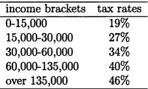
2.1 Structure of 1998 IRPEF tax brackets in Lit ’000 (Lit 1,936.27 = €1). 30 2.2 Tax allowances for dependent spouse and for other dependent relatives
in Lit ’000 (Lit 1,936.27 = € 1) 31
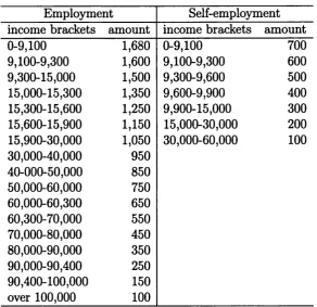
2.3 Tax allowances depending on amount and type of income received in Lit ’000 (Lit 1,936.27 = € 1 ) ... 32
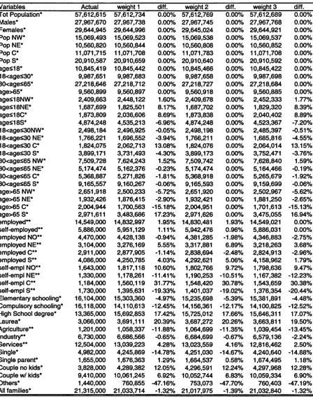
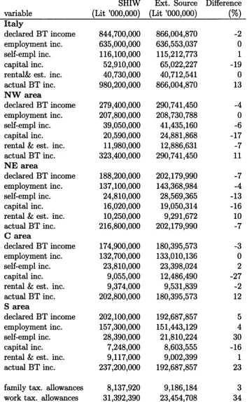
2.4 Grossed-up variables using Banca d ’ltalia (2000) grossing-up weights compared with population totals. *External source: ISTAT (2004). **External source: CNEL (2004)... 35
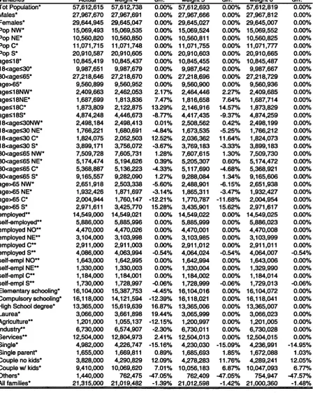
2.5 Grossed-up variables using alternative grossing-up weights compared with population totals. ^External source: ISTAT (2004). **External source: CNEL (2004)... 37 2.6 Grossed-up variables using alternative grossing-up weights compared
with population totals. * External source: ISTAT (2004). ** External
source: CNEL (2004)... 38
2.7 Summary statistics for initial SHIW and final grossing-up weights. . . 39 2.8 Tax evasion estimation for TABEITA98... 41
2.9 Validation of the TABEITA98 output, at the national and area level.
Ext. Sources: Ministero delle Finanze (2002); CNEL (2004) 44
3.1 Abbreviations used in tables and f i g u r e s ... 56 3.2 Actual 1998 and counterfactual structure of IRPEF tax brackets (Lit
3.3 Actual 1998 and counterfactual tax allowances for dependent spouse
(Lit 1 9 3 6 .2 7 = 6 1 )... 72 3.4 Actual 1998 and counterfactual tax allowances for dependent children
and other relatives (Lit 1 9 3 6 .2 7 = 6 1 )... 73 3.5 Actual 1998 and counterfactual tax allowances for employment income.
* is an average. The actual tax allowance (in Lit ’000) was computed
as 851 - [ { v b — 12,400) x 0.78], where yB is BT income... 73
3.6 Self-employment tax allowances. * is an average. The actual tax al lowance (in Lit ’000) was computed as 168-[(2/b — 6,800) x 0.78], where
y s is BT income... 74 3.7 Lorenz curve for different type income ... 75
3.8 Some inequality indices for different type of in c o m e ... 75
4.1 Proportion of households by occupation of the household head . . . . 86 4.2 Occupation of household head if not w orking... 86 4.3 Asymptotic and bootstrap 90% confidence intervals as % of the esti
mate for the sample mean; e = 0 89
4.4 Asymptotic and bootstrap 90% confidence intervals as % of the esti
mate for the sample mean; e = 0 .5 90
4.5 Asymptotic and bootstrap 90% confidence intervals as % of the esti
mate for the sample mean; e = 1 90
4.6 Asymptotic and bootstrap 90% confidence intervals for the 20th per
centile; e = 0 91
4.7 Asymptotic and bootstrap 90% confidence intervals for the 20th per
centile; e = 0 .5 91
4.8 Asymptotic and bootstrap 90% confidence intervals for the 20th per
centile; e = 1 91
4.9 Asymptotic and bootstrap 90% confidence intervals for the 40th per
4.10 Asymptotic and bootstrap 90% confidence intervals for the 40th per
centile; e = 0 .5 ... 92
4.11 Asymptotic and bootstrap 90% confidence intervals for the 40th per centile; e = 1 ... 92
4.12 Asymptotic and bootstrap 90% confidence intervals for the 50th per
centile; e = 0 ... 93 4.13 Asymptotic and bootstrap 90% confidence intervals for the 50th per
centile; e = 0 .5 ... 93
4.14 Asymptotic and bootstrap 90% confidence intervals for the 50th per centile; e = l ... 93
4.15 Asymptotic and bootstrap 90% confidence intervals for the 60th per centile; e = 0 ... 94 4.16 Asymptotic and bootstrap 90% confidence intervals for the 60th per
centile; 6 = 0 .5 ... 94 4.17 Asymptotic and bootstrap 90% confidence intervals for the 60th per
centile; e = l ... 94 4.18 Asymptotic and bootstrap 90% confidence intervals for the 80th per
centile; e = 0 95
4.19 Asymptotic and bootstrap 90% confidence intervals for the 80th per centile; 6 = 0 .5 ... 95
4.20 Asymptotic and bootstrap 90% confidence intervals for the 80th per centile; e = l ... 95
4.21 Asymptotic and bootstrap 90% confidence intervals for the GE(0); e = 0 96
4.22 Asymptotic and bootstrap 90% confidence intervals for the GE(0); e = 0 . 5 ... 97
4.23 Asymptotic and bootstrap 90% confidence intervals for the GE(0); e = 1 97 4.24 Asymptotic and bootstrap 90% confidence intervals for the GE(1); e = 0 97
4.25 Asymptotic and bootstrap 90% confidence intervals for the G E(1); e =
4.27 Asymptotic and bootstrap 90% confidence intervals for the GE(2); e = 0 98
4.28 Asymptotic and bootstrap 90% confidence intervals for the GE(2); e =
0 . 5 ... 99
4.29 Asymptotic and bootstrap 90% confidence intervals for the GE(2); e = 1 99 4.30 MSM: Asymptotic and bootstrap 90% confidence intervals as % of the estimate for the sample mean; e = 0 .5 ... 101
4.31 MSM: Asymptotic and bootstrap 90% confidence intervals as % of the estimate for the 20th percentile; e = 0 .5 ... 101
4.32 MSM: Asymptotic and bootstrap 90% confidence intervals as % of the estimate for the 40th percentile; e = 0 .5 ... 102
4.33 MSM: Asymptotic and bootstrap 90% confidence intervals as % of the estimate for the 50th percentile; e = 0 .5 ... 102
4.34 MSM: Asymptotic and bootstrap 90% confidence intervals as % of the estimate for the 60th percentile; e = 0 .5 ... 103
4.35 MSM: Asymptotic and bootstrap 90% confidence intervals as % of the estimate for the 80th percentile; e = 0 .5 ... 103
4.36 MSM: Asymptotic and bootstrap 90% confidence intervals as % of the estimate for the GE(0); e = 0.5 ... 104
4.37 MSM: Asymptotic and bootstrap 90% confidence intervals as % of the estimate for the GE(1); e = 0 . 5 ... 104
4.38 MSM: Asymptotic and bootstrap 90% confidence intervals as % of the estimate for the GE(2); e = 0 . 5 ... 105
6.1 Decomposition of the population by age g r o u p s ... 139
6.2 Decomposition of the population by household t y p e ... 140
6.3 Decomposition of the population by number of com ponents... 141
6.4 Labor force participation: Total, by sex, by a g e ... 143
6.5 Inequality by different type of in c o m e s ... 155
6.6 Inequality of equivalent household income ... 156
6.8 Counterfactuals using DFL methodology - Base year is 1 9 9 1 ... 171 6.9 Counterfactuals using DFL + Burtelss methodology - Base year is 1991177
6.10 Counterfactuals using Burtless methodology - Base year is 1991 . . . 178
List of Figures
3-1 Analysis of density estimates using different band widths on the whole
sample; in Lit ’000 (Lit 1 9 3 6 .2 7 = 6 1 )... 57 3-2 AT income densities by occupation of the householder, with 90% con
fidence bands; in Lit ’000 (Lit 1936.27=61) ... 58 3-3 Difference between counterfactual AT and actual 1998 AT income den
sities, by occupation of the householder and with different bandwidths;
in Lit ’000 (Lit 1936.27=61)... 59 3-4 Losers and gainers, whole sample; different bandwidhts, 90% confi
dence bands; in Lit ’000 (Lit 1 9 3 6 .2 7 = 6 1 )... 61 3-5 Losers and gainers, by occupation of the householder; Silverman’s
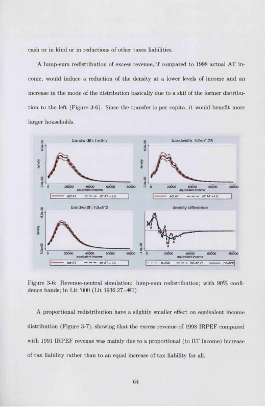
bandwidth, 90% confidence bands; in Lit ’000 (Lit 1936.27=61) . . . 63 3-6 Revenue-neutral simulation: lump-sum redistribution; with 90% con
fidence bands; in Lit ’000 (Lit 1936.27=61) ... 64 3-7 Revenue-neutral simulation: lump-sum redistribution; with 90% con
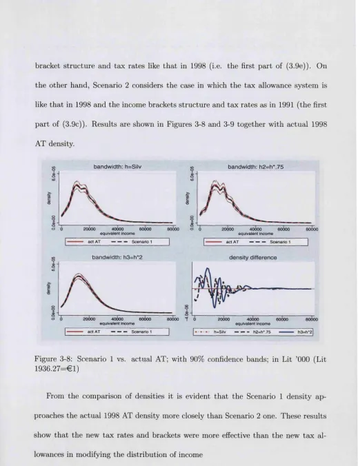
fidence bands; in Lit ’000 (Lit 1936.27=61) ... 65 3-8 Scenario 1 vs. actual AT; with 90% confidence bands; in Lit ’000 (Lit
1936.27=61) ... 67 3-9 Scenario 2 vs. actual AT; with 90% confidence bands; in Lit ’000 (Lit
1936.27=61) ... 68
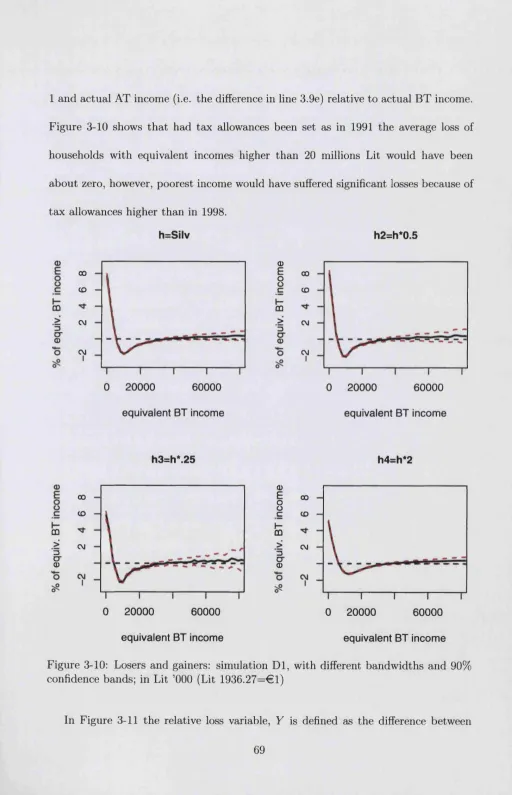
3-10 Losers and gainers: simulation DI, with different bandwidths and 90% confidence bands; in Lit ’000 (Lit 1936.27=61)... 69
3-11 Losers and gainers: simulation D2, with different bandwidths and 90%
6-1 Decomposition of the population by age g r o u p s ... 138
6-2 Decomposition of the population by HH ty p e ... 141
6-3 Decomposition of the population by HH ty p e ... 142
6-4 Labor force participation: Total, by sex, by a g e ... 144
6-5 Frequency of income earners in av. HH or p o p u la tio n ... 146
6-6 Inequality indices, individual (monthly) in co m es... 151
6-7 Inequality indices, individual (monthly) in co m es... 152
6-8 Inequality indices, individual (monthly) in co m es... 153
6-9 Frequency of income earners in av. HH or p o p u la tio n ... 154
6-10 DFL methodology: number of income receivers and number of compo nents in H H ... 166
6-11 DFL methodology: number of income receivers in HH and probability of being p e n sio n ers... 168
6-12 DFL methodology: number of income receivers and probability of fe male in the labor f o r c e ... 169
6-13 Decomposition of the population by s e x ... 170
6-14 Counterfactuals using Burtless m eth o d o lo g y ... 173
6-15 Counterfactuals using Burtless m eth o d o lo g y ... 174
6-16 Counterfactuals using Burtless m eth o d o lo g y ... 175
6-17 Counterfactuals using DFL+Burtless methodology... 176
7-1 t-ratio of Cauchy and infinite-first-moment symmetric Pareto distribu tions ... 192
7-2 t-ratio of symmetric Pareto distributions with 1 < a < 2 ... 193
7-3 t\ Pareto distributions with 0 < a < l ... 193
7-4 of Pareto distributions with 1 < a < 2... 194
7-8 ERP for one-tail test with a sample from a symmetric or a positive
definite Pareto with 1 < a 2... 200
7-9 Test of difference in mean of Pareto distributions with /? = .3... 202
7-10 ts with infinite first moment distributions... 204
7-11 £3 with Pareto distribution with 1 < a < 2 ... 204
A bbreviations
MSM microsimulation model
FES Family Expenditure Study (U.K.)
BT before-tax
AT after-tax
SHIW Survey of Household Income and Wealth (Italy)
IRPEF Imposta sui Redditi delle PErsone Fisiche (personal income
NW North-West
NE North-East
C
Centers
SouthMF Ministero delle Finanze (Italian Ministry of Finance) ISTAT Italian Institute of Statistics
CPI Consumer Price Index
GE Generalized Entropy inequality indices
LIS Luxembourg Income Study
DGP data generating process
EDF empirical distribution function
CDF cumulative distribution function
LFP labor force participation
DF density function
C hapter 1
M icrosim ulation: a to o l for
econom ic analysis
Simulation can be described as a process of imitating the behavior of complex systems,
such as economic or biological systems, a set of tax rules or the computer network of a
large firm: given a set of available information, simulation allows one to build a system
th at imitates the “reality” . Simulation, as a method of solving problems, becomes of
relevance when conventional analytical, numerical, physical or experimental methods
are too expensive, complicated or time demanding.
Simulation models in economics were originally developed by Orcutt (1957) and
Orcutt et a!. (1961) to investigate socioeconomic systems using a microanalytic ap
proach. Economic modelling using simulation was seen as an alternative to aggregate-
type national income models originated by the work of Tinbergen (1939), and input-
output models th at followed the work of Leontief (1951). Tinbergen’s approach uses
timating and testing macroeconomic relationships on the basis of annual or quar
terly time series data of such variables as aggregate consumption and income of the
household sector. Leontief’s approach uses industries as basic components and places
emphasis on the cross-sectional structure of the economy rather than on its dynamic
features. O rcutt’s approach instead develops the most general model in terms of its
statistical structure, since it is developed to include both Tinbergen’s and Leontief’s
models features and to increase details of the micro unit involved (Orcutt et al., 1976).
Since the pioneering work of Orcutt, simulation has played an increasing role in
economic research and has greatly evolved with respect to its initial aims. In Sec
tion 1.1 the role of simulation in economics will be discussed, focusing mainly on
microsimulaton models, i.e. on models th at use microeconomic units as the basis of
their simulations. The following sections will focus mainly on tax-benefit microsimula
tion models, broadly divided in static and dynamic models: Section 1.2 deals with the
former, Section 1.3 with the latter. A distinction is often made between cross-section
and longitudinal dynamic microsimulation models: they will be discussed in Sections
1.3.1 and 1.3.2. In Section 1.4 some issues of particular relevance to microsimulation
modelling will be discussed, namely the grossing-up procedure, the validation and
reliability of microsimulation models. Section 1.5 concludes this chapter.
1.1
M icrosim ulation in econom ics
In recent years, there has been an extensive development of simulation models for
quently as a research tool in economics also thanks to the rapid development of
computers and their easy access to users: fast computers allowed improved accuracy
and the development of more complex simulation systems.
Simulation models are used as conditional forecasting tools to forecast the effect
of shocks or policies on individual units or larger systems. Forecasting can be ex
ante or ex post. In the ex ante case, forecasts are computed on the basis of distinct
conditions described by a given scenario: they are a conditional look into future
developments. In the ex post case, the given real world situation is compared with
alternative interventions (Merz, 1991).
Simulation can be performed at macro or micro level. Macrosimulation models
analyze relationships between national economic sectoral and aggregate variables.
They axe developed using aggregates or sub-aggregates of the totals. They have been
used mainly in government offices for tax forecasting but in the last decades have
been replaced when possible by micro models, which obtain more reliable results the
larger is the complexity of each tax, the diversity of taxpayers and the variation in
the tax base (Eason, 1996, 2000). Macrosimulation models are still used in particular
contexts, such as forecasting of North Sea taxation (Blow et al., 2002). Macrosimu
lation models are developed by central banks to describe long-run equilibrium in the
economy. An example of such models is the Macro Model (MM) at the Bank of Eng
land, which is mainly used by the Monetary Policy Committee to set interest rates
and attain the inflation target. Macromodels are also used in applied general equilib
rium models, which can include detailed scenarios on macroeconomic developments in
goods, changing in trade policies. An example of these complex models is MONASH
for the Australian economy (Meagher, 1996).
Microsimulation models focus directly on micro units such as individuals, house
holds and firms. If these micro units are firms they can be identified by their orga
nization, their occupation structure, the set of products, etc.; if they are individuals
they can be identified by demographic characteristics such as age, sex, occupation,
residence.
Microeconomic models of firms are relatively less common, the main limitation
being in the availability of data for firms. Microsimulation of firms within a model
of the economy was first developed by Eliasson (1978) in a model for Sweden. This
model is a complete micro- to macro-model that contains a selection of the most
important corporate firms, which are simulated in conjunction with residual firms to
replicate the Swedish economy. These models often incorporate production aspects as
well as financial aspects, using a firm in an uncertain and changing environment th at
is assumed to behave with bounded rationality. These models are very demanding in
terms of data and this is one of the main reasons why not all developed economies
have such a model. Among the few exceptions, see van Tongeren (1995) for the Dutch
economy.
Microsimulation models on individuals or households have developed rapidly in
recent decades. Simulation is used in economics mainly to develop counterfactual
analysis to forecast possible effects of different economic policies, but it also serves
in particular situations for generating data that are missing. The structure of a
a simulation model is a set of algebraic equations and decision structures, which can
be characterized as a complex set of “if... then” relations. Relations, procedures and
data can be either completely determined or incorporate random errors. If relations
are all completely specified the simulation is known as deterministic; if randomness
is included the simulation is known as stochastic.
The main aim of microsimulation models based on individual or household data
is to analyze the impact of policy changes on the distribution of some target vari
ables rather than on their mean, as it happens using regression techniques. The
development of microsimulation models on households goes together with increas
ing availability and reliability of micro data sets and improving computer capacity.
Static models generally are based on sample surveys, which provide detailed informa
tion about individual and family characteristics, labor force status, housing status,
earnings. They typically contain the receipt of social security benefits and income
tax liabilities, or incorporate enough information for their calculation. W ith a mi
crosimulation model the immediate distributional impact of fiscal policies, such as
an increase in child benefits, in income tax rates or in the minimum wage, can be
modelled, and estimates of the characteristics of winners and losers and total cost can
be computed. Microsimulation models can also be used to project into the future and
to assess the socio-economic consequences of an ageing population, or of changes in
educational structure and in marriage patterns. In recent years various microsimula
tion modelling methodologies have been developed: some of them will be discussed
in Section 5.3 in the context of inequality decomposition and Chapter 6 will provide
A field of economics where microsimulation has been widely exploited is the analy
sis of the effects of tax-benefit reforms on income, welfare and behavior of individuals.
Until the early 1980s tax-benefit microsimulation models were not widespread and
it was rather common to analyze tax-benefit effects using a range of representative
households. Government agencies and academic departments decided to invest effort
and monetary resources in developing microsimulation models since it was clear that
representative household analysis is unable to give a broad picture of the effect of
the policy on the whole population. For instance, Atkinson and Sutherland (1983)
compared the family composition and circumstances recorded in the UK Family Ex
penditure Survey 1980 with the hypothetical family types used in the Department
of Health and Social Security (DHSS) tax-benefit model. They found th at some 4%
of actual families were covered by the assumption of the complex DHSS hypothet
ical family model. This concern is even more relevant for some of the theoretical
simulation models used to investigate the effects of government policy in a complex
intertemporal setting.
Nowadays virtually all developed countries have at least one model to simulate
changes of taxes and benefits on individual incomes (see among others Mitton et al.,
2000; Gupta and Kapur, 2000; Sutherland, 1994) and after the transition from central
ized planning to a market economy and the consequent need of financing government
policy through taxation, also Eastern and Central European countries showed an in
creased interest in tax-benefit microsimulation models (see for instance Coulter et al.,
1998; Juhasz, 1998). In the European Union the EUROMOD project developed a 15-
impact of changes to personal tax and transfer policy each taking place at either the
national or the European level, to assess the consequences of consolidated social poli
cies and to understand how different policies in different countries may contribute to
common objectives (Sutherland, 2001). The rest of this chapter will mainly focus on
tax-benefit microsimulation models (MSMs).
1.2
Static m icrosim ulation m odels
Static MSMs are based on instantaneous pictures of characteristics of a sample of a
population in a given period. They are appropriate models for the analysis of the
impact of policy changes, where these effects can be deduced, completely or in large
part, from knowledge of the current circumstances of individuals in the sample.
In static MSMs behavioral relations and institutional conditions are varied exoge
nously. Micro-data bases are comprised of a cross-section of micro units in a given
period. These micro units are generally assigned a sampling weight, which allows one
to infer about the population of origin.
Static microsimulation is first developed for the specific period to which the data
relate. A static MSM can then be applied to different time periods using static “aging
procedures” . Such a procedure consists in re-weighting the available information using
given aggregate of another time period. After re-weighting a sample, a new weight will
be assigned to each micro unit, i.e. each micro unit will represent a different number
of units in the whole population. However, the number of observations in the data
A static ageing procedure is the easiest ageing procedure and can be reasonably
applied for short- or medium-run forecasts, where it can reasonably be assumed th at
demographic characteristics of the underlying population do not change significantly.
A static aging procedure involves updating income and wealth data. It is common
to update income and wealth variables using for all units growth in money income
or a price index such as the retail price index (RPI) or the consumer price index.
This solution can lead to important bias. Sutherland (1989) showed th at while in
the period 1982-1988 RPI increased by 32%, the earnings of full-time adult men in
the bottom decile grew by 42% and those in the top decile grew by an average of
64% in the same period. Notwithstanding this limitation, straightforward indexing
by published data is often the only possible way to go, mainly for reasons of data
limitation. Updating bias can be a very limited problem if considered over a short
period of time.
The term “static” may seem limiting when compared to “dynamic” . However, in
some contexts dynamic models are not very useful. In fact, static models allow one
to hold constant a large number of variables so that it becomes possible to isolate
some elements of particular interest. In the setting of fiscal policies, for instance, they
can separate direct effects on income of changing the structure of tax and benefits
from other possible effects (see for instance, Chapter 3). Static models, which are
sometimes also called “arithmetic”, are the building block of more complex models,
such as behavioral or dynamic ones (see among many others, Atkinson and Sutherland
1.2.1
S tatic m icrosim ulation m od els w ith behavioral responses
One of the shortcomings of static MSMs is the assumption that individual behavior
is exogenous. However, many tax and benefit policies are designed specifically to
have behavioral effects. For instance many policy reform are designed to encourage
more labor force participation; other transfer policies may have unintended negative
incentive consequences; government revenues and expenditures calculations may be
misleading if potential behavioral responses are not properly taken into account and
estimated.
The type of static MSMs discussed in this subsection are intended as an improve
ment through the introduction of explicit modelling of behavioral responses to policy
reforms. They hold certain characteristics fixed (such as family composition) but
allow other characteristics to change, like labor force participation and, consequently,
earnings. This type of modelling presents many computational and analytical prob
lems and is nowadays one of the most dynamic field in the microsimulation literature.
To include behavioral response it is necessary to handle complex budget constraints
th at allow each individual’s constraint to be unique, along with the desire to model
heterogeneity. All these issues impose demanding modelling and computer program
ming requirements (Duncan, 2003). In fact, all components of a tax-benefit MSM
have to be closely integrated and, given the large number of sample units involved, it
is important to invest in developing efficient computer routines. Researchers have to
decide about the underlying economic model and its econometric specification. They
observed outcome, and simulating the effects of policies on individual behavior.
MSMs with behavioral responses are developed from a static MSM without be
havioral responses. Since they introduce additional complication to modelling issues,
they also increase their limitations in terms of grossing-up, validation and reliability of
results issues. Moreover they are more demanding in terms of data quality. Most data
sets include fewer information about non-workers than about workers: the researcher
has then to introduce “reasonable” assumptions, which will affect the reliability of the
estimates. Although MSMs with behavioral response have been criticized for being
rather unreliable, particularly in estimating figures of losers and gainers, tax revenue
and overall inequality after-tax reforms (Pudney and Sutherland, 1996), their use has
proved very successful in the labor economics literature, namely in estimating the
labor supply responses to changes in net wages (see, among others Blundell et al.,
1992, 1998; Duncan and Giles, 1996).
1.3
D yn am ic m icrosim ulation m odels
Dynamic MSMs differ from static ones mainly in terms of the ageing procedure.
In dynamic MSMs each micro unit is aged individually using survivor probabilities
estimated empirically. Dynamic models not only include the possibility of death but
introduce events such as marriage, household composition evolution, such as births,
inclusion of other relatives in the household, divorce. Hence, dynamic demographic
ageing will create a new data set whose dimension will typically be different from the
Demographic dynamics will also rises the issue of the inclusion of behavioral re
sponse to demographic changes: for instance, if a child is born it is possible that
the mother’s decision to participate in the labor market will change. However, the
magnitude of behavioral change is difficult to assess due to the widely divergent es
timates of relevant elasticities, and simulations are generally presented for a number
of different estimates (Hagenaars, 1990, p. 31).
It is also debatable whether the elasticities obtained from cross-section data can
be assumed to closely reflect lifetime behavioral response. For instance, there is panel
data evidence that labor force participation decisions are made with a very long time
horizon in mind (Heckman and MaCurdy, 1980, p. 67) and th at future expected
values of variables determined current labor supply decisions (MaCurdy, 1981, 1983).
Therefore it could be th at a higher real wage increases labor force participation in
the short term but life-cycle income will be partly offset by a decision to retire earlier
(Harding, 1990, p. 15). Among dynamic MSMs, the main distinction is between
dynamic cross-section and dynamic longitudinal models.
1.3.1
D yn am ic cross-section m icrosim ulation m od els
Dynamic cross-section MSMs (or dynamic population MSMs) attem pt to project mi
cro units forward through time simulating demographic events such as death, birth,
marriage, divorce, etc. Recently also immigration has been introduced (see for in
stance Walker, 2000). After a main demographic event has been modelled, other
data base for dynamic cross-section MSM is the same as in the static model, i.e. a
random sample of the population.
Dynamic cross-section models are aimed at depicting the future structure of the
population and typically map only a few decades of the lives of individuals from many
age cohorts. They are useful to forecast the future characteristics of the population
and to model the effects of policy changes during the next years or decades.
These models have been mainly applied for analyzing the distributional impacts of
social security system (see, for instance Favreault and Caldwell, 2000; Nelissen, 1996),
the evolution of the pension systems (see Galler, 1996; Eklind et al., 1996; Andreassen
et al., 1996) or lifetime analysis of poverty alleviation programs (see Falkingham and
Harding, 1996).
1.3.2
D yn am ic longitudinal m icrosim ulation m od els
In a dynamic longitudinal MSMs (or dynamic cohort MSMs) the aging process is
as in the cross-section models but only one cohort is aged rather than the entire
population. In general, one cohort is aged from birth to death so th at a whole life
cycle of one cohort is simulated. The same life cycle profiles can be generated with
dynamic cross-section models, however it would be inefficient if lifetime circumstances
of one or two cohorts are of interest.
Dynamic longitudinal models are generally used for analyzing lifetime earnings
and income distributions, to assess the lifetime incidence of taxes and government
process than cross-section MSMs and are easier to model since they restrict attention
to the demographics and socio-economic dynamics of a single cohort rather to all
cohorts in a population.
1.3.3
L im itation s o f dynam ic m icrosim ulation m od els
Dynamic models, as extensions of static MSMs, present additional limitations.
Dynamic MSMs axe more data hungry: they need additional information to esti
mate demographic changes to be included in dynamic models. Ideally these data sets
include death rates by age, sex and socio-economic status, marriage rates by age, sex,
education level and previous marital status; divorce rates by age, sex, duration of
marriage, and number of age of children; attendance rates at primary, secondary and
tertiary levels by age, sex, parental socio-economic status and previous education;
labor force participation rate by age, sex, education, marital status, age of children,
duration of current employment and of unemployment spells, etc. Moreover, cross-
section data are not usually adequate for setting the parameters in dynamic models.
For instance, the probability of transition between states can only be obtained from
longitudinal data (Harding, 1990).
Since it is rare for a data set to be suitable for every kind of analysis, dynamic
models generally rely on whatever piece of data is available, using matching techniques
to put information together. This procedure is done at the expense of reducing the
accuracy of the models and of requiring frequent updates.
error is likely to happen in estimating survivor and transition probabilities and demo
graphic changes. An additional source of error arises from the simulation of transitions
to different states and survivor probabilities: since these events are obtained using
Monte Carlo simulations, different simulations introduce different state-transition in
the single micro unit. The model sensitivity to different simulation can be assessed by
using a large number of replications. However, this is often difficult to perform since
dynamic models (and especially dynamic cross-section models) require huge comput
ing resources to run: the characteristics of the micro units in the initial year have to
be stored and the final analysis is thus frequently based upon a very large number of
observations.
1.4
Issues in m icrosim ulation m odelling
Among the various challenges that microsimulation modelling poses, the issues of
grossing-up, validation and reliability are worth additional attention. They have
been studied mainly in the context of static MSM, though they are of relevance for
all types of microsimulation models.
1.4.1 G rossing-up
The procedure of grossing-up is concerned with generating figures to cover the popu
lation being modelled from the data set under use. The procedure should adjust for
differences between the sample data and the characteristics of the population to be
The grossing-up procedure is basically aimed at adjusting the data set to reflect
differential non-response between different groups in the sample. It involves stratify
ing the sample, by some relevant characteristics, after the data have been collected
and applying known proportions. This procedure is also sometimes referred to as
post-stratification (see for instance Atkinson and Micklewright (1983)).
The grossing-up procedure consists in assigning to each unit in a sample of di
mension N a weight Pj with j = 1,..., N , such that some chosen statistics of interest
calculated on the weighted sample coincide with the population statistics. The pro
cedure is trivial if we want to reconcile the sample with the population using only one
discrete statistic, s* with k = 1,...K , such as family types or income ranges. In this
case, we compute the probability of having the characteristic s* in the sample, say
P(sjfc), and make it equal to the probability of having the same characteristic in the
population, say p(s*). If the dimension of the sample and of the population are N
and n respectively, then the grossing-up weight is Pj = n p ( s k ) /N P ( s k ) , i.e. the size
of the cell with characteristic s* in the population divided by the size of the cell with
characteristic s* in the sample. If more variables are considered for the grossing-up
procedure it should be necessary to consider the interactions between the different
variables, i.e. consider the joint distribution of the control variables considered. How
ever, this conflicts with available information from external sources, th at in general,
do not report the joint distribution of population variables but only the totals for
each variable. For instance, it is possible to know the total number of single-parent
families and the total number of self-employed in the population but not how many
on the weights pj are far less stringent than in the “full information” case we would
have if the joint distribution were known, and in general there are many possible
sets of weights Pj achieving the desired adjustment. To choose among them Atkinson
et al. (1988) suggest the requirement th at given a data set of dimension N , with
original sampling weights qj, j = 1,2, ...,1V, the set of grossing-up weights Pj have
the least deviation from original weights, qj. The original weights could reflect the
sampling procedure or be uniform. Both grossing-up and initial weights have to sum
up to the population size: Qj = YhPj ~ 71 • If original and sample weights sum up
to the sample dimension, they first have to be multiplied by n / N . It is then common
practice to impose the condition that the new weights minimize the distance from
initial weights. Hollenbeck (1976) proposed to use as a measure of distance the half
of the squared sum of the difference between final and initial weights. However, in
order to avoid negative weights, Atkinson et al. (1988) suggest minimizing a measure
of distance derived from information theory (Theil, 1967; Cowell, 1980):
d(p,q) = ^ lPjlog(%-'j (1.1)
As for the optimal number of control totals to be included, no result is currently avail
able. Although it is more common to face the problem of not having enough external
sources than to have too many, Sutherland (1989, p. 15) warns on the risk of increas
ing the variance of weights since the larger the number of control totals becomes,
the smaller the number of observations in each “cell’ (i.e. with each combination of
Atkinson et al. (1988) applied their methodology1 to TAXMOD, a MSM for the
UK, and compared their results with what could be obtained with uniform weights, i.e.
multiplying the sampling weights by n / N . The grossed-up results were significantly
more plausible. The conclusion from their analysis is th at the use of uniform weights
can be seriously misleading.
1.4.2
V alidation
Model validation is a task consisting of two distinct but related aspects. First it con
sists in comparing the primary data set to external data from a number of sources.
This procedure is complementary to grossing-up in that detailed information not used
as control totals are used as control data after grossing-up has been performed. Sec
ondly, validation involves looking at the results of the model’s output and analyzing
them in relation to estimates published elsewhere. If the external source for validation
is using the same sample this validation ends up in a comparison of different models.
If validation is with estimates using different data sets, the comparison analyzes the
robustness of results of both estimates. Hence, model validation is an exercise with a
broader scope than grossing-up since it deals with model construction as well as its
output (Hope, 1988).
However, model validation is also less easy to perform than grossing-up, at least
as for the comparison of different estimates: it presumes that there is at least another
model with a comparable level of accuracy to compare results with.
1.4.3
R eliab ility
Although MSMs are widely used nowadays few authors working in this field have paid
explicit attention to the statistical reliability of MSM output. MSMs typically produce
summary statistics such as average income, income percentile, inequality indices,
number of gainers and losers after a policy simulation. This output is an estimate
of effects of changes in some policy instruments and, as well as any other statistical
estimate, it should be accompanied by a standard error or confidence intervals. MSMs,
as all survey-based models, can be affected by measurement and misreporting errors.
They can also introduce peculiar errors such as errors in updating data to a later year,
bad or no specification of behavioral response and market adjustments, stochastic
simulation error. However, simulated figures are often quoted without standard error
or confidence intervals and it is often hard to distinguish reliable results from those
badly affected by sampling or other source of error. The main reason for not providing
confidence intervals or standard error to MSM output is probably due to the technical
problems involved in their calculation.
Pudney and Sutherland (1994) provide the first contribution on the reliability
of MSMs. They investigate the asymptotic sampling properties of a set of typical
simulation results, focusing on the sampling error assuming that finite population
corrections can be avoided. They used equivalent income to account for economies of
scale in the family or household. Although equivalence scales are non linear transfor
mations, Pudney and Sutherland simply assume that errors are normally distributed
standard error, where ca/2 is the a / 2 critical value for the normal distribution. Their
application on 1998 Family Expenditure Study (FES, U.K.) data using a static MSM
without behavioral response shows that the basic process of simulation seems rear
sonably reliable. However, they find th at while some statistics are estimated with
acceptable precision, others, like number of gainers and losers, poverty and inequality
indices, can have a wide margin of sampling error and suggest th at there should be
some doubt about the reliability of some widely-quoted simulation results.
Even more pessimistic conclusions are reached in Pudney and Sutherland (1996)
where asymptotic confidence intervals are estimated in a static MSM th at incorporates
a multinomial logit model of female labor supply. The resulting confidence intervals
allow errors associated with sampling variability, parameter estimation and stochastic
simulation. Pudney and Sutherland found th at the sampling error is the main source
of variability for most summary statistics, but that the measures describing the impact
of policy on female participation are very uncertain and may be of no practical use
to economists, mainly because of the variability of parameter estimates.
Chapter 4 contributes to the analysis of static MSM reliability using the bootstrap
to compute confidence intervals. The bootstrap is considered for two main reasons:
(a) it allows one to remove the hypothesis of infinite population to compute confidence
intervals using a simulation-based methodology rather than finite sample corrections,
and (b) there is a growing body of literature showing th at bootstrap often performs
better, or not worse, than asymptotic approximation in small samples. It is found
th at bootstrap confidence intervals are in general less conservative than asymptotic
of the complex non-linear setting of MSMs, to derive the exact or Monte Carlo finite
population confidence intervals is a formidable task and it is not possible to evaluate
the improved precision of bootstrap confidence intervals compared with asymptotic
confidence intervals. However, the generally good performance of the bootstrap in
finite samples should increase the concern about the reliability of estimates on par
ticular sub-samples of widely used surveys. It was also found th at MSMs itself do not
necessarily make confidence intervals larger. In some cases, summary statistics on
simulated incomes have narrower confidence intervals, as percentage of the computed
statistic, than before the tax-benefit simulation. These results show th at concerns in
sampling error with MSMs are sometimes misplaced: it is not microsimulation that
necessarily makes the estimation less reliable. A poor coverage of the population
of some current surveys is often the main cause of error and improvement in data
collection should be pursued.
1.5
C onclusion
Microsimulation models and, in particular tax-benefit microsimulation models are
powerful tools for analyzing effects of demographic trends or to assess the effects on
living standards of various public policies. However they cannot provide an answer
for every question and must be handled with care. A great deal of attention should
also be devoted to the presentation and analysis of data. In Chapter 3 non-parametric
density estimation is proposed to increase the understanding of MSM output.
should never be just the production of numbers: grossing-up, validation procedures
and confidence interval estimation should be carefully addressed. A reliable MSM will
also increase the credibility of a modelling technique th at has only recently started
being extensively exploited by academics.
A great deal of attention should also be devoted to improve data collection, since
Chapter 2
A static tax-benefit
m icrosim ulation m odel for Italy
MSMs are powerful research tools with high fixed costs. In recent years the devel
opment of personal computers allowed single researchers to build their own MSM,
however, building a MSM to simulate the complexity of economic systems still often
requires team work. In the case of tax-benefit MSMs good programmers, who manage
to develop fast computer codes, have to work together with experts of the tax and
benefit legislation and of its implementation problems, and with econometricians who
axe able to analyze and treat data with rigor. For this thesis it was decided to look
at Italian models for personal interest and also because my knowledge of the Italian
tax-benefit system is deeper than that of any other national system, although the
results of this and the following two chapters should also be of interest for non-Italian
MSMs. The starting point for any MSM is the choice of the data set: the more it is
the more reliable the model becomes. Section 2.1 describes and discusses the main
limitations of the 1998 SHIW data set, which is used for the MSM presented in this
chapter.
To gain full access to a MSM, a new model had to be developed. When this
project started no model using 1998 SHIW data set had been completed. The MSM
developed for this thesis is TABEITA98: it was constructed using 1998 SHIW data
set and STATA software, partly following the structure of Dirimod951. The main
features of TABEITA98 are briefly described in Section 2.2. Section 2.3 describes
how the tax base was built from the available data set and Section 2.4 deals with the
issue of grossing-up the model. Section 2.5 shows how the model was employed to
estimate tax evasion and how these findings were used to validate the model. Section
2.6 concludes.
2.1
T h e data set for Italian M SM s
The data set used in this chapter is the Survey of Household Income and Wealth
(SHIW) published by the Bank of Italy and based on interviews run in 1998. This
data set will also be used in Chapters 3, 4 and 7. The SHIW is a long standing survey:
it was started in the mid 1960s, was run about annually up to 1987, henceforth about
every two years. The Bank of Italy paid particular attention to improve the quality of
the data. For instance since 1995 an increasing number of interviews were performed
using a computer to check consistency of answers and particular attention was paid
in formulating questions as clearly as possible with several trial interviews (Banca
d ’ltalia, 2000, p.29). At present the SHIWs are the main, if not the only, data set
for Italian household MSMs and among the most frequently used for any kind of
household income analysis at the national level in Italy (for a review of other data
sets, see Brandolini, 1999).
The 1998 data set collects detailed micro data for about 7,147 households and
20,901 individuals on disposable income, consumption, labor market, monetary and
financial variables. The sample was drawn in two stages (municipalities and house
holds) with the stratification of the primary sampling units (municipalities) by units
and size, to make it representative of the national population. Within each stratum,
all municipalities with population of more than 40,000 were selected, while smaller
towns were randomly included. Households were then selected randomly and a sam
pling weight, defined as the inverse of the probability of inclusion of each household
in the sample, was attached to each observation. Since 1989 a number of households
who had been interviewed previously have been interviewed again, to start producing
a panel data set. Although in the present and following chapters the panel will not
be considered, it has an effect on the probability of a household being included in the
sample. These issues have been addressed and resolved by the Bank of Italy, which
provides a set of appropriate sampling weights. Data are checked before release: the
strategy is either to drop the interview for the whole household if missing d ata can
not be reasonably inferred from other characteristics of the individual/household or
to impute the missing data, often using regression models to forecast missing vari
imputation is less 0.1% for most variables (Banca d’ltalia, 2000, p.35).
2.1.1
Som e lim itation s o f th e database
Among the limitations of the SHIW data set some affect any analysis of Italian
household income, some others are specifically of interest for the reliability of MSMs.
A first limitation of the data set is the low rate of response. Participation in
the survey is voluntary and not paid. Although all households were granted total
anonymity, in 1998 only 52.6% of contacted households agreed to being interviewed.
The low rate of response can cause a selectivity bias as some households seem to be
more likely to refuse an interview. In fact, the likelihood of accepting an interview
decreases with increases in income, wealth and education of the household head, and
the size of the town of residence (Banca d ’ltalia, 2000, p.31). In order to mitigate
the selectivity bias some measures are adopted, such as the replacement of refusing
households with others from the same town. Some estimations of the selectivity bias
on incomes recorded in SHIW show that the underestimation of household income is
on average rather limited (Cannari and D’Alessio (1992) estimate it at about 5%).
Other limitations of this data set include the fact that the household is interviewed
rather than the family. This leads to an overestimation of the average number of
components, which cannot be corrected at all since the relevant information is missing.
The interviews include only recall questions, i.e. questions referring to the previous
year, reducing the precision of the reporting. An alternative approach would be to ask
but it was discarded to keep a reasonable rate of response and to avoid approximations
th at come from extending the week or month to cover the whole year. Finally, data
do not include information about people who do not have a registered dwelling or are
in a hospital or other kind of institution.
As for the limitations which are more relevant for MSMs, the main one refers
to the type of income recorded: it refers to disposable income, excluding taxes and
social contributions paid and benefit received. Hence, the first role of a MSM is to
simulate the before-tax income before introducing any other policy simulation. This
feature implies that, in contrast to other MSMs, no simulation error2 can be properly
assessed (for the U.K. see Pudney and Sutherland (1994)).
2.2
Structure o f th e m odel
The MSM developed for this thesis is TABEITA98, a TAx-BEnefit microsimulation
model on ITAlian 1998 SHIW data. TABEITA98 refers to 1998 personal income
taxation (IRPEF and “imposte sostitutive”)3 net of social contributions. TABEITA98
is a static model without behavioral response. It can be described as a deterministic
transformation of a given sample into a new one. Let y A and y B be the vectors
of after-tax (AT) and before-tax (BT) income, respectively: the former vector is
obtained from the latter through a tax transformation, say r*, i = 1,2..., iV, where N
is the number of individuals in the sample. Since the data are net of taxes and social
2The simulation error is defined as the difference between the simulated after-tax income, obtained applying the MSM to the declared before-tax income, and the declared after-tax income.
contributions, the first role of the model is to recover individual BT income:
y ? = r r1(y? ) (2 .1)
for alH = 1, ...N . There are two major complications here. First, the tax transfor
mation Tj is not the same for all individuals. Personal income taxation in Italy is on
individual base; the amount of tax each individual has to pay depends on the type
of incomes she receives and her family characteristics. For instance, arrears do not
enter the personal income tax (IRPEF) base: they are taxed with a proportional tax
rate while work and pension income is taxed with progressive tax rates; there are
several tax allowances which depend on a set of individual and family characteristics,
such as the number of dependent children, whether the spouse is dependant, whether
income comes from self-employment, employment or pension, etc. Secondly, the tax
transformation in (2.1) is highly non linear. This implies th at y s has to be obtained
numerically, by recursive approximations. The tax transformation, 7*, used to recover
y B is obtained from the 1998 tax code. Various assumptions about take-up rates of
tax allowances could be introduced, however no uncertainty is considered here. Al
though the analysis of benefits take-up is a relevant issue in countries where welfare
programs are widespread4 in Italy there are no generalized unemployment benefit,
income maintenance or house benefit schemes. The issue of non take-up is limited to
tax allowances and tax deductions which do not involve issues of stigma or psycho
logical dependency and is then less relevant. Moreover, this choice, together with the
idea of not considering behavioral responses, allowed the model to be as simple and
robust as possible5.
In this model the main assumptions are that (a) the sample is representative of
the population and contains enough details for simulation, (b) the tax and benefit
legislation, 7*, is perfectly known by the individual and applied without error. Al
though the first assumption is granted by the Bank of Italy who produced the data,
the second is meant to keep variability to a minimum. An alternative solution would
be to randomly include errors in the model assessing the relevance of such changes
in the MSM. Here, instead, only systematic errors leading to under-reporting are
considered and treated as tax evasion or tax avoidance in Section 2.5; involuntary
under-reporting is assumed to be off-setting with involuntary over-reporting errors.
The probability of programming mistakes is kept to a minimum with a number of
checks and a validation procedure (see Section 2.5).
TABEITA98 is developed in four different modules using Stata 7 on a personal
computer. The first module involves the preparation of the data base, and in par
ticular the data consistency checks. The second is the grossing-up procedure. The
third involves an estimation of tax evasion to correct the underreporting of certain
population groups and validation of the output. The last deals with the simulation of
alternative scenarios. The first three stages will be briefly presented in the following
sections. Chapter 3 will provide an illustration of simulations th at can be performed
with TABEITA98.
The model allows one to compute the amount of tax allowances, of tax base
deductions, the amount of personal income tax paid, the BT income6, transfers and
pensions not liable of personal income tax. All incomes can be computed at the
individual and household level, allowing for different equivalence scales.
2.3
B uilding th e ta x base
As a first step the model has to put together the different types of incomes to build
the tax base. TABEITA98 was initially built and developed following Dirimod95,
using 1995 SHIW data (Mantovani, 1998)7. Analysis of data is performed starting
from employment, pension, self-employment incomes and rents. They all form the
IRPEF tax base. During the reconstruction of the tax base, the data imputation of
the Bank of Italy is analyzed: it appears to be particularly relevant especially for
self-employment and rental income. Although the Bank of Italy does not explain in
detail how the data imputation is performed and what kind of additional information
are known and used, imputed data are used here.
Once all the components o